Generate Synthetic Signals Using Conditional GAN

This example uses:

This example shows how to generate synthetic pump signals using a conditional generative adversarial network.

Generative adversarial networks (GANs) can be used to produce synthetic data that resembles real data input to the networks. GANs are useful when simulations are computationally expensive or experiments are costly. Conditional GANs (CGANs) can use data labels during the training process to generate data belonging to specific categories.

This example treats simulated signals obtained by a pump Simulink™ model as the "real" data that plays the role of training data set for a CGAN. The CGAN uses 1-D convolutional networks and is trained using a custom training loop and a deep learning array. In addition, this example uses principal component analysis (PCA) to visually compare the characteristics of generated and real signals.

CGAN for Signal Synthesis

CGANs consist of two networks that train together as adversaries:

Generator network — Given a label and random array as input, this network generates data with the same structure as the training data observations corresponding to the same label. The objective of the generator is to generate labeled data that the discriminator classifies as "real."
Discriminator network — Given batches of labeled data containing observations from both training data and generated data from the generator, this network attempts to classify the observations as "real" or "generated." The objective of the discriminator is to not be "fooled" by the generator when given batches of both real and generated labeled data.

Ideally, these strategies result in a generator that generates convincingly realistic data corresponding to the input labels and a discriminator that has learned strong features characteristic of the training data for each label.

Load Data

The simulated data is generated by the pump Simulink model presented in the Multi-Class Fault Detection Using Simulated Data example. The Simulink model is configured to model three types of faults: cylinder leaks, blocked inlets, and increased bearing friction. The data set contains 1575 pump output flow signals, of which 760 are healthy signals and 815 have a single fault, combinations of two faults, or combinations of three faults. Each signal has 1201 signal samples with a sample rate of 1000 Hz.

Download and unzip the data in your temporary directory, whose location is specified by MATLAB® tempdir command. If you have the data in a folder different from that specified by tempdir, change the directory name in the following code.

% Download the data
dataURL = 'https://ssd.mathworks.com/supportfiles/SPT/data/PumpSignalGAN.zip';
saveFolder = fullfile(tempdir,'PumpSignalGAN'); 
zipFile = fullfile(tempdir,'PumpSignalGAN.zip');
if ~exist(fullfile(saveFolder,'simulatedDataset.mat'),'file')
    websave(zipFile,dataURL);
    % Unzip the data
    unzip(zipFile,saveFolder)
end

The zip file contains the training data set and a pretrained CGAN:

simulatedDataset — Simulated signals and their corresponding categorical labels
GANModel — Generator and discriminator trained on the simulated data

Load the training data set and standardize the signals to have zero mean and unit variance.

load(fullfile(saveFolder,'simulatedDataset.mat')) % load data set
meanFlow = mean(flow,2);
flowNormalized = flow-meanFlow;
stdFlow = std(flowNormalized(:));
flowNormalized = flowNormalized/stdFlow;

Healthy signals are labeled as 1 and faulty signals are labeled as 2.

Define Generator Network

Define the following two-input network, which generates flow signals given 1-by-1-by-100 arrays of random values and corresponding labels.

The network:

Projects and reshapes the 1-by-1-by-100 arrays of noise to 4-by-1-by-1024 arrays by a custom layer.
Converts the categorical labels to embedding vectors and reshapes them to a 4-by-1-by-1 arrays.
Concatenates the results from the two inputs along the channel dimension. The output is a 4-by-1-by-1025 array.
Upsamples the resulting arrays to 1201-by-1-by-1 arrays using a series of 1-D transposed convolution layers with batch normalization and ReLU layers.

To project and reshape the noise input, use the custom layer projectAndReshapeLayer, attached to this example as a supporting file. The projectAndReshapeLayer object upscales the input using a fully connected layer and reshapes the output to the specified size.

To input the labels into the network, use an imageInputLayer object and specify a size of 1-by-1. To embed and reshape the label input, use the custom layer embedAndReshapeLayer, attached to this example as a supporting file. The embedAndReshapeLayer object converts a categorical label to a one-channel array of the specified size using an embedding and a fully connected operation. For categorical inputs, use an embedding dimension of 100.

% Generator Network

numFilters = 64;
numLatentInputs = 100;
projectionSize = [4 1 1024];
numClasses = 2;
embeddingDimension = 100;

layersGenerator = [
    imageInputLayer([1 1 numLatentInputs],'Normalization','none','Name','in')
    projectAndReshapeLayer(projectionSize,numLatentInputs,'proj');
    concatenationLayer(3,2,'Name','cat');
    transposedConv2dLayer([5 1],8*numFilters,'Name','tconv1')
    batchNormalizationLayer('Name','bn1','Epsilon',5e-5)
    reluLayer('Name','relu1')
    transposedConv2dLayer([10 1],4*numFilters,'Stride',4,'Cropping',[1 0],'Name','tconv2')
    batchNormalizationLayer('Name','bn2','Epsilon',5e-5)
    reluLayer('Name','relu2')
    transposedConv2dLayer([12 1],2*numFilters,'Stride',4,'Cropping',[1 0],'Name','tconv3')
    batchNormalizationLayer('Name','bn3','Epsilon',5e-5)
    reluLayer('Name','relu3')
    transposedConv2dLayer([5 1],numFilters,'Stride',4,'Cropping',[1 0],'Name','tconv4')
    batchNormalizationLayer('Name','bn4','Epsilon',5e-5)
    reluLayer('Name','relu4')
    transposedConv2dLayer([7 1],1,'Stride',2,'Cropping',[1 0],'Name','tconv5')
    ];

dlnetGenerator = dlnetwork(layersGenerator,'Initialize',false);

layers = [
    imageInputLayer([1 1],'Name','labels','Normalization','none')
    embedAndReshapeLayer(projectionSize(1:2),embeddingDimension,numClasses,'emb')];

dlnetGenerator = addLayers(dlnetGenerator,layers);
dlnetGenerator = connectLayers(dlnetGenerator,'emb','cat/in2');
dlnetGenerator = initialize(dlnetGenerator);

Plot the network structure for the generator.

plot(dlnetGenerator)

Define Discriminator Network

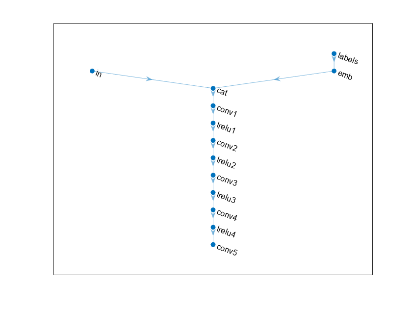
Define the following two-input network, which classifies real and generated 1201-by-1 signals given a set of signals and their corresponding labels.

This network:

Takes 1201-by-1-by-1 signals as input.
Converts categorical labels to embedding vectors and reshapes them to a 1201-by-1-by-1 arrays.
Concatenates the results from the two inputs along the channel dimension. The output is a 1201-by-1-by-1025 array.
Downsamples the resulting arrays to scalar prediction scores, which are 1-by-1-by-1 arrays, using a series of 1-D convolution layers with leaky ReLU layers with a scale of 0.2.

% Discriminator Network

scale = 0.2;
inputSize = [1201 1 1];

layersDiscriminator = [
    imageInputLayer(inputSize,'Normalization','none','Name','in')
    concatenationLayer(3,2,'Name','cat')
    convolution2dLayer([17 1],8*numFilters,'Stride',2,'Padding',[1 0],'Name','conv1')
    leakyReluLayer(scale,'Name','lrelu1')
    convolution2dLayer([16 1],4*numFilters,'Stride',4,'Padding',[1 0],'Name','conv2')
    leakyReluLayer(scale,'Name','lrelu2')
    convolution2dLayer([16 1],2*numFilters,'Stride',4,'Padding',[1 0],'Name','conv3')
    leakyReluLayer(scale,'Name','lrelu3')
    convolution2dLayer([8 1],numFilters,'Stride',4,'Padding',[1 0],'Name','conv4')
    leakyReluLayer(scale,'Name','lrelu4')
    convolution2dLayer([8 1],1,'Name','conv5')];

dlnetDiscriminator = dlnetwork(layersDiscriminator,'initialize',false);

layers = [
    imageInputLayer([1 1],'Name','labels','Normalization','none')
    embedAndReshapeLayer(inputSize,embeddingDimension,numClasses,'emb')];

dlnetDiscriminator = addLayers(dlnetDiscriminator,layers);
dlnetDiscriminator = connectLayers(dlnetDiscriminator,'emb','cat/in2');
dlnetDiscriminator = initialize(dlnetDiscriminator);

Plot the network structure for the discriminator.

plot(dlnetDiscriminator)

Train Model

Train the CGAN model using a custom training loop. Loop over the training data and update the network parameters at each iteration. To monitor the training progress, display generated healthy and faulty signals using two fixed arrays of random values to input into the generator as well as a plot of the scores of the two networks.

For each epoch, shuffle the training data and loop over mini-batches of data.

For each mini-batch:

Generate a dlarray (Deep Learning Toolbox) object containing an array of random values for the generator network.
For GPU training, convert the data to a gpuArray (Parallel Computing Toolbox) object.
Evaluate the model gradients using dlfeval (Deep Learning Toolbox) and the helper function modelGradients.
Update the network parameters using the adamupdate (Deep Learning Toolbox) function.

The helper function modelGradients takes as input the generator and discriminator networks, a mini-batch of input data, and an array of random values, and returns the gradients of the loss with respect to the learnable parameters in the networks and the scores of the two networks. The loss function is defined in the helper function ganLoss.

Specify Training Options

Set the training parameters.

params.numLatentInputs = numLatentInputs;
params.numClasses = numClasses;
params.sizeData = [inputSize length(labels)];
params.numEpochs = 1000;
params.miniBatchSize = 256;

% Specify the options for Adam optimizer
params.learnRate = 0.0002;
params.gradientDecayFactor = 0.5;
params.squaredGradientDecayFactor = 0.999;

Set the execution environment to run the CGANs on the CPU. To run the CGANs on the GPU, set executionEnvironment to "gpu" or select the "Run on GPU" option in Live Editor. Using a GPU requires Parallel Computing Toolbox™. To see which GPUs are supported, see GPU Computing Requirements (Parallel Computing Toolbox).

executionEnvironment = "cpu";
params.executionEnvironment = executionEnvironment;

Skip the training process by loading the pretrained network. To train the network using the trainGAN helper function on your computer, set trainNow to true or select the "Train CGAN now" option in Live Editor.

trainNow = false;
if trainNow
    % Train the CGAN
    [dlnetGenerator,dlnetDiscriminator] = trainGAN(dlnetGenerator, ...
        dlnetDiscriminator,flowNormalized,labels,params); %#ok
else
    % Use pretrained CGAN (default)
    load(fullfile(tempdir,'PumpSignalGAN','GANModel.mat')) % load data set
end

The training plot below shows an example of scores of the generator and discriminator networks. To learn more about how to interpret the network scores, see Monitor GAN Training Progress and Identify Common Failure Modes (Deep Learning Toolbox). In this example, the scores of both the generator and discriminator converge close to 0.5, indicating that the training performance is good.

Synthesize Flow Signals

Create a dlarray object containing a batch of 2000 1-by-1-by-100 arrays of random values to input into the generator network. Reset the random number generator for reproducible results.

rng default

numTests = 2000;
ZNew = randn(1,1,numLatentInputs,numTests,'single');
dlZNew = dlarray(ZNew,'SSCB');

Specify that the first 1000 random arrays are healthy and the rest are faulty.

TNew = ones(1,1,1,numTests,'single');
TNew(1,1,1,numTests/2+1:end) = single(2);
dlTNew = dlarray(TNew,'SSCB');

To generate signals using the GPU, convert the data to gpuArray objects.

if executionEnvironment == "gpu"
    dlZNew = gpuArray(dlZNew);
    dlTNew = gpuArray(dlTNew);
end

Use the predict function on the generator with the batch of 1-by-1-by-100 arrays of random values and labels to generate synthetic signals and revert the standardization step that you performed on the original flow signals.

dlXGeneratedNew = predict(dlnetGenerator,dlZNew,dlTNew)*stdFlow+meanFlow;

Signal Feature Visualization

Unlike images and audio signals, general signals have characteristics that make them difficult for human perception to tell apart. To compare real and generated signals or healthy and faulty signals, you can apply principal component analysis (PCA) to the statistical features of the real signals and then project the features of the generated signals to the same PCA subspace.

Feature Extraction

Combine the original real signal and the generated signals in one data matrix. Use the helper function helperExtractFeature to extract the feature including common signal statistics such as the mean and variance as well as spectral characteristics.

idxGenerated = 1:numTests;
idxReal = numTests+1:numTests+size(flow,2);

XGeneratedNew = squeeze(extractdata(gather(dlXGeneratedNew)));
x = [XGeneratedNew single(flow)];

features = zeros(size(x,2),14,'like',x);

for ii = 1:size(x,2)
    features(ii,:) = helperExtractFeature(x(:,ii));
end

Each row of features corresponds to the features of one signal.

Modify the labels for the generated healthy and faulty signals as well as real healthy and faulty signals.

L = [squeeze(TNew)+2;labels.'];

The labels now have these definitions:

1 — Generated healthy signals
2 — Generated faulty signals
3 — Real healthy signals
4 — Real faulty signals

Principal Component Analysis

Perform PCA on the features of the real signals and project the features of the generated signals to the same PCA subspace. W is the coefficient and Y is the score.

% PCA via svd
featuresReal = features(idxReal,:);
mu = mean(featuresReal,1);
[~,S,W] = svd(featuresReal-mu);
S = diag(S);
Y = (features-mu)*W;

From the singular vector S, the first three singular values make up 99% of the energy in S. You can visualize the signal features by taking advantage of the first three principal components.

sum(S(1:3))/sum(S)

ans = single

0.9965

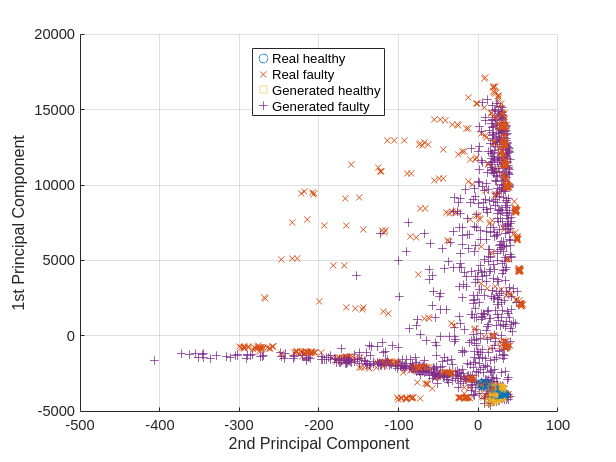
Plot the features of all the signals using the first three principal components. In the PCA subspace, the distribution of the generated signals is similar to the distribution of the real signals.

idxHealthyR = L==1;
idxFaultR = L==2;

idxHealthyG = L==3;
idxFaultG = L==4;

pp = Y(:,1:3);

figure
scatter3(pp(idxHealthyR,1),pp(idxHealthyR,2),pp(idxHealthyR,3),'o')
xlabel('1st Principal Component')
ylabel('2nd Principal Component')
zlabel('3rd Principal Component')
hold on
scatter3(pp(idxFaultR,1),pp(idxFaultR,2),pp(idxFaultR,3),'x')
scatter3(pp(idxHealthyG,1),pp(idxHealthyG,2),pp(idxHealthyG,3),'s')
scatter3(pp(idxFaultG,1),pp(idxFaultG,2),pp(idxFaultG,3),'+')
view(160,30)
legend('Real healthy','Real faulty','Generated healthy','Generated faulty', ...
    'Location','Best')
hold off

To better capture the difference between the real signals and generated signals, plot the subspace using the first two principal components.

view(90,-90)

Healthy and faulty signals lie in the same area of the PCA subspace regardless of their being real or generated, demonstrating that the generated signals have features similar to those of the real signals.

Predict Labels of Real Signals

To further illustrate the performance of the CGAN, train an SVM classifier based on the generated signals and then predict whether a real signal is healthy or faulty.

Set the generated signals as the training data set and the real signals as the test data set. Change the numeric labels to character vectors.

LABELS = {'Healthy','Faulty'};
strL = LABELS([squeeze(TNew);labels.']).';

dataTrain = features(idxGenerated,:);
dataTest = features(idxReal,:);

labelTrain = strL(idxGenerated);
labelTest = strL(idxReal);

predictors = dataTrain; 
response = labelTrain;
cvp = cvpartition(size(predictors,1),'KFold',5);

Train an SVM classifier using the generated signals.

SVMClassifier = fitcsvm( ...
    predictors(cvp.training(1),:), ...
    response(cvp.training(1)),'KernelFunction','polynomial', ...
    'PolynomialOrder',2, ...
    'KernelScale','auto', ...
    'BoxConstraint',1, ...
    'ClassNames',LABELS, ...
    'Standardize',true);

Use the trained classifier to obtain the predicted labels for the real signals. The classifier achieves a prediction accuracy above 90%.

actualValue = labelTest;
predictedValue = predict(SVMClassifier,dataTest);
predictAccuracy = mean(cellfun(@strcmp,actualValue,predictedValue))

predictAccuracy = 
0.9467

Use a confusion matrix to view detailed information about prediction performance for each category. The confusion matrix shows that, in each category, the classifier trained based on the generated signals achieves a high degree of accuracy.

figure
confusionchart(actualValue,predictedValue)

Case Study

Compare the spectral characteristics of real and generated signals. Due to the nondeterministic behavior of GPU training, if you train the CGAN model yourself, your results might differ from the results in this example.

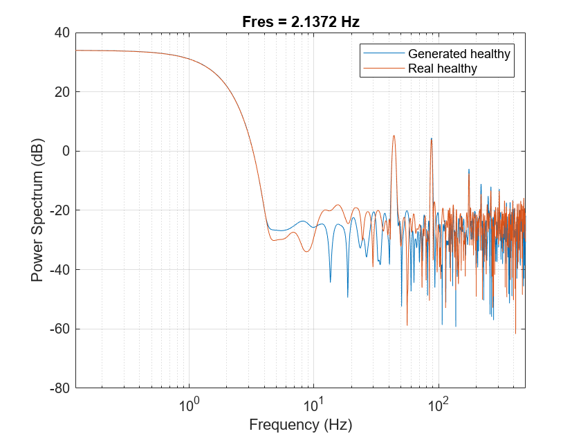
The pump motor speed is 950 rpm, or 15.833 Hz, and since the pump has three cylinders the flow is expected to have a fundamental at 3 times 15.833 Hz, or 47.5 Hz, and harmonics at multiples of 47.5 Hz. Plot the spectrum for one case of the real and generated healthy signals. From the plot, the generated healthy signal has relatively high power values at 47.5 Hz and 2 times 47.5 Hz, which is exactly the same as the real healthy signal.

Fs = 1000;
pspectrum([x(:,1) x(:,2006)],Fs)
set(gca,'XScale','log')
legend('Generated healthy','Real healthy')

If faults exist, resonances will occur at the pump motor speed, 15.833 Hz, and its harmonics. Plot the spectra for one case of real and generated faulty signals. The generated signal has relatively high power values at around 15.833 Hz and its harmonics, which is similar to the real faulty signal.

pspectrum([x(:,1011) x(:,2100)],Fs)
set(gca,'XScale','log')
legend('Generated faulty','Real faulty')

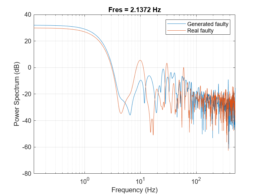
Plot spectra for another case of real and generated faulty signals. The spectral characteristics of the generated faulty signals do not match the theoretical analysis very well and are different from the real faulty signal. The CGAN can still be possibly improved by tuning the network structure or hyperparameters.

pspectrum([x(:,1001) x(:,2600)],Fs)
set(gca,'XScale','log')
legend('Generated faulty','Real faulty')

Computation Time

The Simulink simulation takes about 14 hours to generate 2000 pump flow signals. This duration can be reduced to about 1.7 hours with eight parallel workers if you have Parallel Computing Toolbox™.

The CGAN takes 1.5 hours to train and 70 seconds to generate the same amount of synthetic data with an NVIDIA Titan V GPU.