Remaining Useful Life Estimation of a DC-Link Capacitor in a Power Converter
This example shows the design and implementation of a remaining useful life (RUL) estimation algorithm for an aluminum electrolytic DC-link capacitor in an AC-DC-AC power converter system. The degradation data of the DC-link capacitor is generated using a Simulink® model and Simscape™ Electrical™ blocks.
The degradation profiles of the DC-link capacitor capacitance and equivalent series resistance (ESR) are injected into the corresponding Series RLC Branch block parameters in the model over a simulated lifetime of 24 months. The resulting training data set (i.e., features and the health indicator) for the RUL algorithm is generated through the use of a simulation ensemble. Accessing logged simulation data using a simulation ensemble simplifies the processing and analysis of the degradation data for feature extraction and the subsequent training of the RUL algorithm.
AC-DC-AC Power Converter
A 60 Hz, 25 kV source feeds a 50 Hz, 50 kW load through an AC-DC-AC converter. The 60 Hz, 600 V voltage obtained at the secondary of the Wye/Delta transformer is first rectified using a six-pulse-diode bridge. The filtered DC voltage is applied to an IGBT two-level inverter generating a 50 Hz power output, which then drives the 380 Vrms AC load. The IGBT inverter uses Pulse Width Modulation (PWM) at a 2 kHz carrier frequency. The circuit is discretized at a sample time of 20 s (50 kHz).
mdl = 'pdmACDCACConverter';
open_system(mdl)
Warning: Unrecognized function or variable 'CloneDetectionUI.internal.CloneDetectionPerspective.register'.

The DC-link capacitor, which is used as a filter at the output of the rectifier, has an initial capacitance of 5000 F and an ESR of 40 m. The role of the DC-link capacitor in the power converter is to suppress large voltage fluctuations and current ripples arising from the switching behavior of the inverter.
Electrolytic DC-Link Capacitor Failures
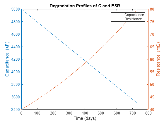
Aluminum electrolytic capacitors degrade over time because of aging, mechanical vibrations, large temperature variations during operation, and evaporation of the electrolyte within the aluminum case. The capacitance and ESR typically degrade linearly and exponentially over time according to the following relationships, respectively [1]:
For electrolytic DC-link capacitors, the generally accepted failure threshold is a 30% percent reduction in capacitance or a 100% increase in ESR, so that
at the time of failure, .
C0 = 5000e-6;
ESR0 = 40e-3;

Cf = 0.7*C0;
ESRf = 2.0*ESR0;
In this example, the degradation of the capacitance and the ESR until failure is simulated over a lifetime of 24 months in order to generate sufficient degradation data and subsequently create the training data set (features) for the RUL model.
Tf = 2*365;
t = (0:Tf)';
C = C0-(C0-Cf)*t/Tf;
ESR = ESR0*exp(log(ESRf/ESR0)*t/Tf);
Plot the degradation profiles for the capacitance and ESR:
figure
title('Degradation Profiles of C and ESR')
xlabel('Time (days)')

yyaxis left
plot(t,1e6*C,'--')
ylabel('Capacitance (\muF)')

yyaxis right
plot(t,1e3*ESR,'-.')
ylabel('Resistance (m\Omega)')

legend('Capacitance', 'Resistance')

Generate Degradation Data Using Simulink and Simscape
The RUL algorithm uses features extracted from the degradation data, which you obtain by simulating the power converter model over the lifetime of the DC-link capacitor. The model measures the voltage and current on one of the phases of the load, the voltage and current across the DC-link capacitor, and the voltage on one of the phases at the inverter output.
Simulate Component Degradation
The power converter model is configured with variables that control the capacitance and ESR of the DC-link capacitor. By varying the Model Workspace variables (C and ESR), you can create degradation data over the lifetime of the DC-link capacitor.
Use an array of Simulink.SimulationInput objects to define a number of simulation scenarios. For example, you can choose an array of values for the two model variables to represent the degradation of the DC-link capacitor over time and then create a Simulink.SimulationInput object for each combination of these model variable values. Capture the degraded component values once every 30 days using a for-loop.
siminputs = [];
for k = 1:30:numel(t)
  siminput = Simulink.SimulationInput(mdl);
  siminput = siminput.setVariable('C',C(k),'Workspace',mdl);
  siminput = siminput.setVariable('ESR',ESR(k),'Workspace',mdl);
  siminputs = [siminputs,siminput]; %#ok<AGROW>
end
This code creates 25 simulation inputs from the vectors of degradation variable values stored in variables C and ESR, corresponding to one set of measurements every 30 days over the two-year lifetime of the simulated test system.
With the array of Simulink.SimulationInput objects defined, use the generateSimulationEnsemble function to run the simulations. The generateSimulationEnsemble function configures the model to save logged data to files, use the timetable format for signal logging, and store the Simulink.SimulationInput objects in the saved files as additional metadata. The function returns a status flag indicating whether the simulations completed successfully.
folder = fullfile(pwd,'Data');
if ~exist(folder,'dir')
  mkdir(folder)
else
  delete(fullfile(folder,'*.mat'))
end
[ok,e] = generateSimulationEnsemble(siminputs,folder);
[26-Jun-2024 13:10:24] Running simulations...
[26-Jun-2024 13:10:44] Completed 1 of 25 simulation runs
[26-Jun-2024 13:10:47] Completed 2 of 25 simulation runs
[26-Jun-2024 13:10:49] Completed 3 of 25 simulation runs
[26-Jun-2024 13:10:51] Completed 4 of 25 simulation runs
[26-Jun-2024 13:10:54] Completed 5 of 25 simulation runs
[26-Jun-2024 13:10:55] Completed 6 of 25 simulation runs
[26-Jun-2024 13:10:57] Completed 7 of 25 simulation runs
[26-Jun-2024 13:10:59] Completed 8 of 25 simulation runs
[26-Jun-2024 13:11:00] Completed 9 of 25 simulation runs
[26-Jun-2024 13:11:02] Completed 10 of 25 simulation runs
[26-Jun-2024 13:11:03] Completed 11 of 25 simulation runs
[26-Jun-2024 13:11:05] Completed 12 of 25 simulation runs
[26-Jun-2024 13:11:07] Completed 13 of 25 simulation runs
[26-Jun-2024 13:11:08] Completed 14 of 25 simulation runs
[26-Jun-2024 13:11:10] Completed 15 of 25 simulation runs
[26-Jun-2024 13:11:11] Completed 16 of 25 simulation runs
[26-Jun-2024 13:11:13] Completed 17 of 25 simulation runs
[26-Jun-2024 13:11:15] Completed 18 of 25 simulation runs
[26-Jun-2024 13:11:17] Completed 19 of 25 simulation runs
[26-Jun-2024 13:11:19] Completed 20 of 25 simulation runs
[26-Jun-2024 13:11:22] Completed 21 of 25 simulation runs
[26-Jun-2024 13:11:26] Completed 22 of 25 simulation runs
[26-Jun-2024 13:11:28] Completed 23 of 25 simulation runs
[26-Jun-2024 13:11:31] Completed 24 of 25 simulation runs
[26-Jun-2024 13:11:37] Completed 25 of 25 simulation runs
The generateSimulationEnsemble logs the simulation results for each run. Create a simulation ensemble to process and analyze the simulation results using the simulationEnsembleDatastore command.
ens = simulationEnsembleDatastore(folder)
ens =
  simulationEnsembleDatastore with properties:

           DataVariables: [7×1 string]
    IndependentVariables: [0×0 string]
      ConditionVariables: [0×0 string]
       SelectedVariables: [7×1 string]
                ReadSize: 1
              NumMembers: 25
          LastMemberRead: [0×0 string]
                   Files: [25×1 string]
Simulation ensemble contains the data from all the signals logged during simulations as well as some metadata associated with each simulation.
ens.SelectedVariables
ans = 7×1 string
    "Idclink"
    "Iload"
    "SimulationInput"
    "SimulationMetadata"
    "Vdclink"
    "Vinv"
    "Vload"
Preprocess Simulation Results
For analysis, use only the voltage and current measurements across the capacitor and the load. These signals are more likely to contain features indicative of the degradation of the DC-link capacitor over its lifetime. Specify these measurements in the SelectedVariables property of the ensemble.
ens.SelectedVariables = ["Iload";"Vload";"Vdclink";"Idclink"];
data = read(ens)
data=1×4 table
           Iload                  Vload                 Vdclink                Idclink
    ___________________    ___________________    ___________________    ___________________

    {10001×1 timetable}    {10001×1 timetable}    {10001×1 timetable}    {10001×1 timetable}
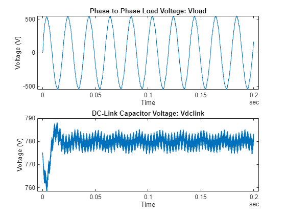
Extract the signals from the data returned for the first ensemble member and plot them to allow a visual inspection of the data.
figure;
subplot(211);
Vload = data.Vload{1};
plot(Vload.Time,Vload.Data)
title('Phase-to-Phase Load Voltage: Vload')
xlabel('Time')
ylabel('Voltage (V)')

subplot(212)
Vdclink = data.Vdclink{1};
plot(Vdclink.Time,Vdclink.Data)
title('DC-Link Capacitor Voltage: Vdclink')
xlabel('Time')
ylabel('Voltage (V)')
The DC-Link Capacitor Voltage plot shows that there are initial transients for up to 50 ms during the simulation. These transients, which are due to the initial conditions of the model, must be ignored so that you use only the steady-state segments of the signals for further analysis. To process all the simulation ensemble members, use the hasdata command to apply the prepareData_dclink function to all the simulation data. This command removes the signal transients that are less than 50 ms from the beginning of all logged signals.
ens.DataVariables = unique([ens.DataVariables;"Iload_reduced";"Vload_reduced";"Vdclink_reduced";"Idclink_reduced"]);
reset(ens)
while hasdata(ens)
  data = read(ens);
  shortData = prepareData_dclink(data);
  writeToLastMemberRead(ens,shortData);
end

reset(ens)
ens.SelectedVariables = ["Iload_reduced";"Vload_reduced";"Vdclink_reduced";"Idclink_reduced"];
data = read(ens)
data=1×4 table
      Iload_reduced         Vload_reduced        Vdclink_reduced       Idclink_reduced
    __________________    __________________    __________________    __________________

    {7501×1 timetable}    {7501×1 timetable}    {7501×1 timetable}    {7501×1 timetable}
After removing the transients, plot a short segment of the DC-link capacitor voltage and current signals for every member of the ensemble using the hasdata and read commands:
figure
reset(ens)
while hasdata(ens)
  data = read(ens);

  subplot(211)
  Vdclink_reduced = data.Vdclink_reduced{1};
  plot(Vdclink_reduced.Time,Vdclink_reduced.Data)
  hold on

  subplot(212)
  Idclink_reduced = data.Idclink_reduced{1};
  plot(Idclink_reduced.Time,Idclink_reduced.Data)
  hold on
end

subplot(211)
xlim(seconds([0,0.005]))
hold off
title('Segments of DC-Link Capacitor Voltages')
xlabel('Time')
ylabel('Voltage (V)')

subplot(212)
xlim(seconds([0,0.005]))
hold off;
title('Segments of DC-Link Capacitor Currents')
xlabel('Time')
ylabel('Current (A)')

The voltage across the DC-link capacitor seems to show more variation over the lifetime of the capacitor. Therefore, the Vdclink_reduced signal of the ensemble members will likely be a good candidate for feature extraction.
Live Remaining Useful Life Estimation with Simulation-in-the-Loop
In order to train and implement an RUL model, you will need to extract a number of diagnostic features and combine some of those features to construct a scalar health indicator (HI). The health indicator will be the input to the RUL model for training and prediction. Therefore, the HI needs to be a reliable indicator of the overall degradation of the system.
Extracting Features
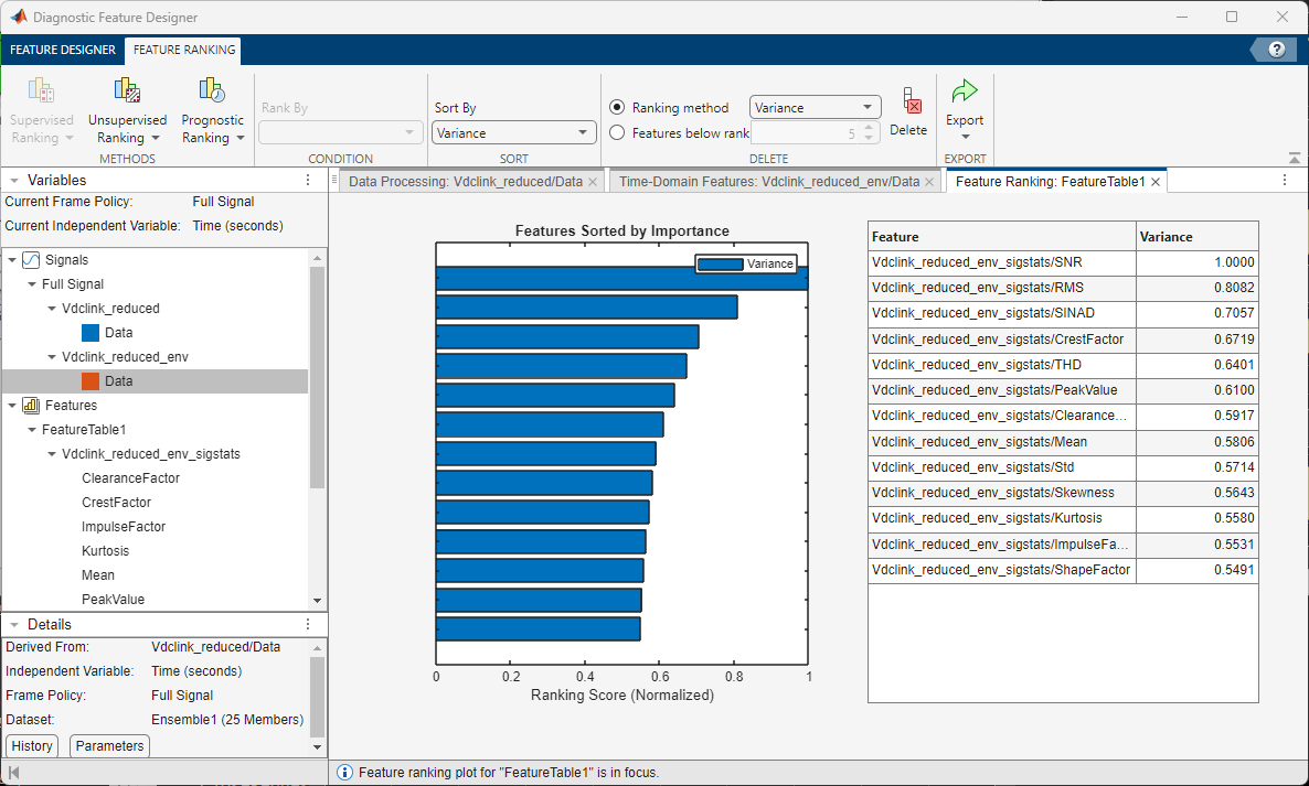
The Diagnostic Feature Designer app was used to create and rank a number of features extracted from the logged signals. You can launch the Diagnostic Feature Designer app using the following command, import the simulation file ensemble ens into the app by clicking New Session, and select only the Vdclink_reduced variable of the ensemble for data processing and feature extraction:
%app1 = diagnosticFeatureDesigner;In this example, we first applied Signal Envelope data processing (with a bandpass filter of 2000 Hz center frequency and 200 Hz bandwidth) upon the shortened DC-link capacitor voltage signals. Signal enveloping helps separate the high-frequency content in the signals that are due to the PWM driver from the low-frequency content that carries more relevant information about the degradation behavior of the DC-link capacitor.

We have then extracted various Signal Features (i.e., basic statistics) from the signal envelope of the DC-link capacitor voltage measurements.

Finally, the resulting signal features were ranked using the Unsupervised Ranking method of Variance (using 50% Correlation Importance and meanvar Normalization Scheme as parameters) to see which features would be good candidates (if used individually) for predicting the degradation of the DC-link capacitor.

After creating various features from the logged signals, the code generation capability of the app was used to generate the diagnosticFeatures_dclink function that encapsulates all the computations needed to generate the same set of ranked features as obtained in the app.
It is important to make sure that the rows of the resulting feature table are sorted in the same order of the successive simulations of the degradation of the system. Therefore, sort the feature table rows to match the simulation number embedded in the name of ensemble data files. The feature table now contains the predictive features that you can use to construct a reliable health indicator and train the RUL model.
featureTable = diagnosticFeatures_dclink(ens);

files = ens.Files;
tokens = regexp(files,'(\d+).mat','tokens');
I = cellfun(@(c)double(c{1}),tokens);
[~,J] = sort(I);

featureTable = featureTable(J,:)
featureTable=25×13 table
Vdclink_reduced_env_sigstats/ClearanceFactor Vdclink_reduced_env_sigstats/CrestFactor Vdclink_reduced_env_sigstats/ImpulseFactor Vdclink_reduced_env_sigstats/Kurtosis Vdclink_reduced_env_sigstats/Mean Vdclink_reduced_env_sigstats/PeakValue Vdclink_reduced_env_sigstats/RMS Vdclink_reduced_env_sigstats/SINAD Vdclink_reduced_env_sigstats/SNR Vdclink_reduced_env_sigstats/ShapeFactor Vdclink_reduced_env_sigstats/Skewness Vdclink_reduced_env_sigstats/Std Vdclink_reduced_env_sigstats/THD
____________________________________________ ________________________________________ __________________________________________ _____________________________________ _________________________________ ______________________________________ ________________________________ __________________________________ ________________________________ ________________________________________ _____________________________________ ________________________________ ________________________________
64.342 7.454 29.152 38.808 1.225 35.711 4.7908 12.257 16.52 3.911 5.9618 4.6319 -14.296
63.156 7.4539 28.952 38.824 1.2334 35.71 4.7908 12.255 16.516 3.8841 5.9629 4.6296 -14.296
61.985 7.4539 28.748 38.841 1.2422 35.71 4.7907 12.254 16.512 3.8567 5.964 4.6272 -14.296
60.827 7.4537 28.541 38.858 1.2512 35.709 4.7907 12.253 16.508 3.829 5.9651 4.6248 -14.296
59.683 7.4536 28.33 38.875 1.2604 35.708 4.7907 12.252 16.505 3.8009 5.9662 4.6223 -14.297
58.553 7.4534 28.117 38.893 1.27 35.707 4.7908 12.25 16.502 3.7724 5.9674 4.6197 -14.297
57.438 7.4531 27.901 38.911 1.2798 35.707 4.7908 12.249 16.497 3.7435 5.9685 4.6171 -14.297
56.336 7.4528 27.681 38.929 1.2899 35.706 4.7909 12.248 16.494 3.7142 5.9697 4.6143 -14.297
55.249 7.4524 27.459 38.948 1.3003 35.705 4.791 12.247 16.492 3.6846 5.9708 4.6115 -14.297
54.176 7.452 27.234 38.967 1.311 35.704 4.7912 12.246 16.489 3.6546 5.972 4.6087 -14.298
53.118 7.4514 27.005 38.987 1.3221 35.703 4.7914 12.245 16.486 3.6242 5.9731 4.6057 -14.298
52.074 7.4508 26.774 39.006 1.3334 35.702 4.7916 12.244 16.481 3.5934 5.9743 4.6027 -14.298
51.044 7.4502 26.54 39.026 1.3451 35.701 4.7919 12.243 16.479 3.5624 5.9755 4.5995 -14.298
50.029 7.4494 26.303 39.047 1.3572 35.699 4.7922 12.242 16.477 3.531 5.9766 4.5963 -14.299
49.029 7.4485 26.064 39.067 1.3696 35.698 4.7926 12.242 16.476 3.4992 5.9778 4.5931 -14.299
48.043 7.4476 25.822 39.088 1.3824 35.697 4.7931 12.241 16.474 3.4672 5.9789 4.5897 -14.299
⋮
Train RUL Prediction Model
We have used the Health Indicator Designer app to construct a health indicator for training the RUL model and predicting the RUL of the DC-link capacitor. You can launch the Health Indicator Designer app using the following command:
%app2 = healthIndicatorDesigner;
After creating a health indicator from the most relevant features, the deployment code generation capability of the app was used to generate the healthIndicator_dclink function that encapsulates the computations needed to generate the scalar health indicator that Health Indicator Designer modeled.
HI = healthIndicator_dclink(featureTable);
The health indicator data along with the corresponding simulation times (once every 30 days) become the training data for the RUL model:
trainingData = timetable(HI, 'VariableNames', {'HealthIndicator'}, 'RowTimes', days(0:30:Tf))
trainingData=25×1 timetable
      Time      HealthIndicator
    ________    _______________

    0 days          0.96562
    30 days         0.92839
    60 days         0.89098
    90 days         0.85339
    120 days        0.81562
    150 days        0.77769
    180 days        0.73697
    210 days        0.69861
    240 days        0.66013
    270 days         0.6215
    300 days        0.58273
    330 days        0.53826
    360 days        0.49927
    390 days        0.46043
    420 days         0.4212
    450 days        0.38189
      ⋮
In this example, we have only a single simulated run-to-failure data set for training the RUL model. To simulate multiple run-to-failure data sets, we simply perturb the original training data with a small amount of Gaussian noise with a variance of 0.1:
trainingData2 = trainingData;
trainingData2.HealthIndicator = HI .* (1+sqrt(0.1)*randn(size(HI)));
A linear degradation model is first initialized with a number of parameter values and the training data sets are used to fit the model parameters to the training data.
rul = linearDegradationModel( ...
  'Theta', -0.0014, ... % 1/(2*365)
  'ThetaVariance', 1, ...
  'NoiseVariance', 1, ...
  'SlopeDetectionLevel', 0.1, ...
  'LifeTimeVariable', "Time", ...
  'LifeTimeUnit', "days", ...
  'DataVariables', "HealthIndicator");
rul.UserData.Threshold = 0.0;
fit(rul, {trainingData, trainingData2})
rul
rul =
  linearDegradationModel with properties:

                    Theta: -0.0014
            ThetaVariance: 4.6686e-09
      SlopeDetectionLevel: 0.1000
                    Prior: [1×1 struct]
            NoiseVariance: 0.0426
    SlopeDetectionInstant: []
       CurrentMeasurement: 0
                      Phi: 1.0318
     InitialLifeTimeValue: []
     CurrentLifeTimeValue: []
         LifeTimeVariable: "Time"
             LifeTimeUnit: "days"
            DataVariables: "HealthIndicator"
                 UserData: [1×1 struct]
              UseParallel: 0
Real-Time Prediction of Remaining Useful Lifetime
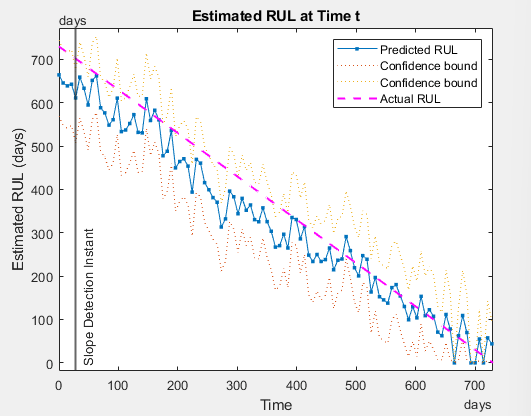
Execute the following commands in the Command Window to run simulations with the Simulink model now acting as the digital twin of an actual power converter and visualize the RUL predictions of the DC-link capacitor. The estimateRUL_dclink function runs a simulation of the digital twin once every 7 simulated days using the degraded capacitance and ESR values augmented with additional Gaussian noise to imitate real-life degradation uncertainties.
estimateRUL_dclink(rul, t, C, ESR, mdl)

hold on
plot(t, t(end) - t, '--', 'Color', 'm', 'LineWidth', 1.5)
set(gca, 'XLim', days([0 t(end)]))
legend('Predicted RUL','Confidence bound','Confidence bound','Actual RUL')
In an actual deployment of the RUL prediction algorithm, the signal data would be measured by voltage and current sensors on the power converter hardware and features would be extracted from those signals, which would then be fed to the RUL algorithm as the health indicator input.
Until the RUL model detects a significant degradation slope change, the RUL predictions are unreliable. After this initial transition period (i.e., the slope detection instant), the RUL prediction converges quickly to the theoretical (actual) RUL value towards a final lifetime value of 2 years.

The RUL model fit and its predictions can be improved by using more training (feature) data sets constructed from run-to-failure data of actual power converter systems or by trying different RUL models such as the exponential degradation model.
References
Yuege Zhou, Xuerong Ye and Guofu Zhai, "Degradation model and maintenance strategy of the electrolytic capacitors for electronics applications", 2011 Prognostics and System Health Management Conference, Shenzhen, China, 2011, pp. 1-6, doi: 10.1109/PHM.2011.5939474.
See Also
Health Indicator
Designer | linearDegradationModel | exponentialDegradationModel
