Main Content

Health Indicator Designer

Interactively transform a set of features into a single composite health indicator that can be used to predict the remaining useful life (RUL) of a machine

Since R2024a

Description

The Health Indicator Designer app allows you to fuse a set of features into a single health indicator (HI) that represents the state of health for the overall system. You can use this single indicator to simplify condition monitoring and RUL predictions in RUL applications.

The app generates MATLAB® code that encapsulates the construction of the HI, which has the general form of a scalar linear regression equation.

H(t) = a0 + a1f1(t) + a2f2(t) + … + anfn(t)

Here, the ai terms are the coefficients that weight the feature contributions. The fi terms are the values of the individual features at time t. a0 is the intercept value. H is typically normalized to a range of [0,1] or [1, 0].

To use the app, you import a feature table that contains an ordered set of features that are computed from measured or simulated data, such as a feature table you export from Diagnostic Feature Designer. You also specify a target profile that represents the degradation profile that you expect the system to follow. The app provides parameters that you can adjust, and plots that show the fit results for the current set of parameters. The various parameters let you control the number of features that the HI incorporates and the mean squared error (MSE) of the fit of the HI to the target.

The goal is to design an HI that incorporates the fewest features possible to achieve the error performance that you require.

For more information on the app parameters and the plot contents, see the corresponding items in the Parameters section.

For information on the algorithms that the app uses, see Algorithms.

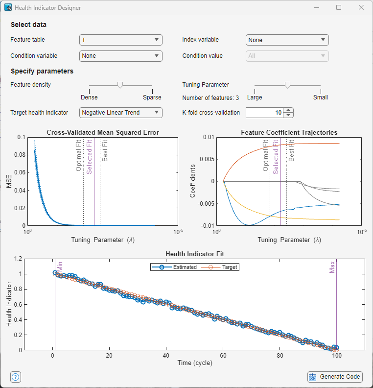
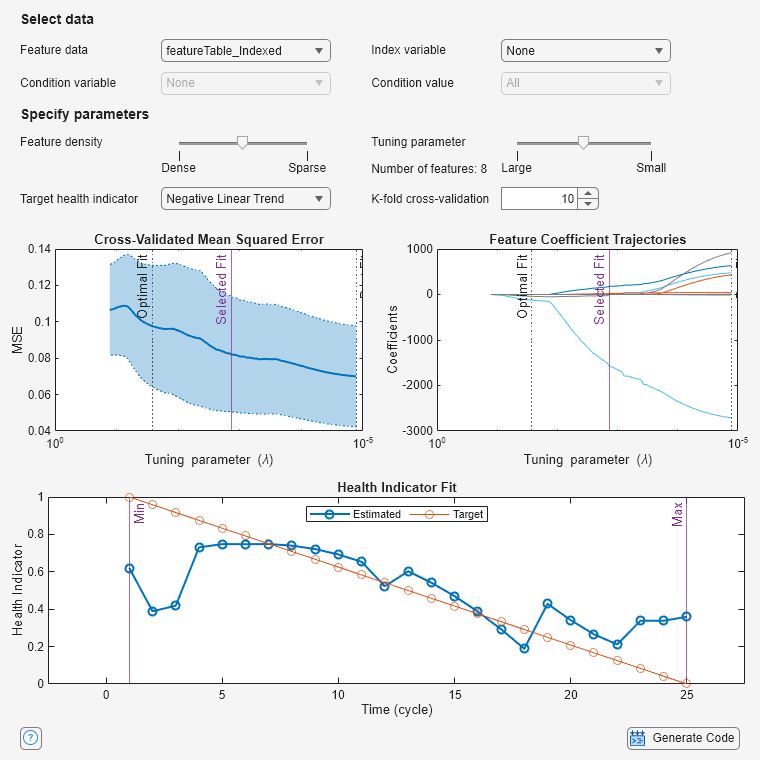
Health Indicator Designer app. From top to bottom, the app contains data selection options, design parameters, and plots of mean squared error, feature coefficient trajectories, and health indicator fit.

Open the Health Indicator Designer App

  • MATLAB toolstrip: On the Apps tab, under Control System Design and Analysis, click the app icon.

  • MATLAB command prompt: Enter healthIndicatorDesigner.

Examples

expand all

Explore ways to use Health Indicator Designer to fuse multiple features into a single health indicator.

Load the data T, which is a timetable that contains feature values for six features which each originate from one of two machines.

load FeatureTableTX T

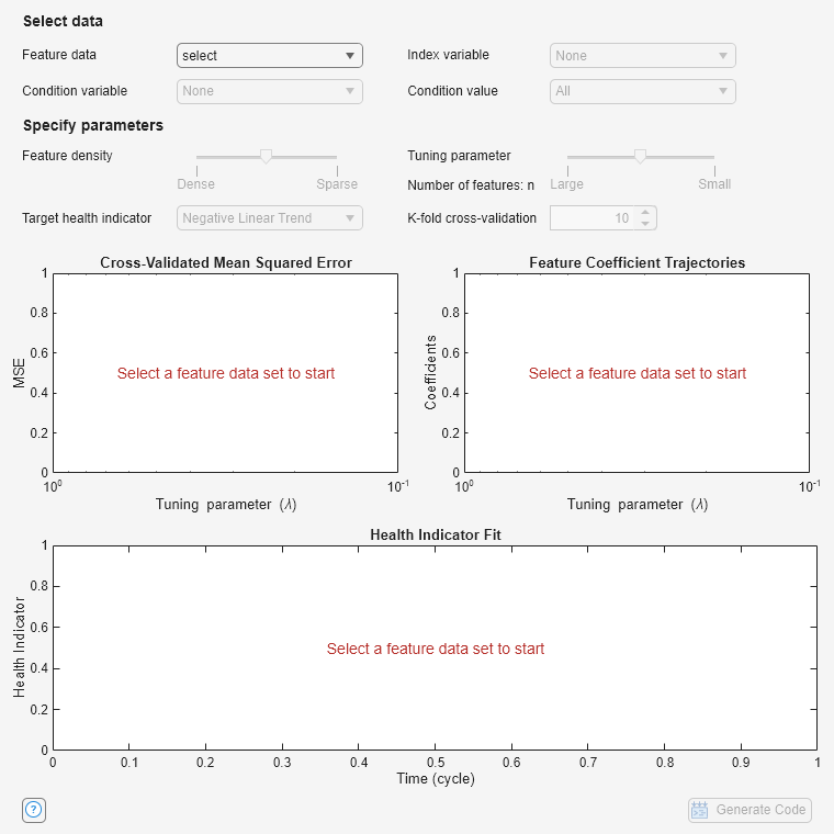
Open the Health Indicator Designer app.

healthIndicatorDesigner

Figure Health Indicator Designer contains 3 axes objects and another object of type uigridlayout. Axes object 1 with title Health Indicator Fit, xlabel Time (cycle), ylabel Health Indicator contains an object of type text. Axes object 2 with title Feature Coefficient Trajectories, xlabel Tuning parameter (\lambda), ylabel Coefficients contains an object of type text. Axes object 3 with title Cross-Validated Mean Squared Error, xlabel Tuning parameter (\lambda), ylabel MSE contains an object of type text.

Evaluate Initial Model

Set Feature table to T. Retain the setting of Negative Linear Trend for Target health indicator. Note that Number of features is 3, which the app computes for the default HI model for T.

The app uses the current set of parameters to plot information about the HI model. You can pause on a trajectory point to obtain feature and coordinate information as a data tip.

The x-axis for both plots is the tuning parameter λ. λ ranges from high to low. The Feature Coefficient Trajectories plot on the right shows the values of the coefficients of the HI model as you move λ across the x-axis range. The higher the coefficient is, the more contribution the feature makes to the HI value. When the coefficient is equal to zero, the feature is excluded completely from the HI model.

The vertical line with the label Selected Fit indicates the current position of λ. You can see that at this point, three features have significant trajectories, and three features are at 0. You can expect the model to include three features for this configuration, which is consistent with the value of Number of Features you saw in the Specify parameters section.

The Cross-Validated Mean Squared Error on the left shows the mean squared error and the variance with respect to the target health indicator, which is plotted beneath the error and trajectories plots.

To view numerical information for this HI model, click Generate Code. The code includes the following information, which is consistent with the plotted trajectories.

% Regression parameters
intercept = 1.03603;
coefficients = [...
    -0.00672674; ...
    0.00826181; ...
    -0.008131; ...
    ];
% Health indicator
HI = intercept + x * coefficients;

Use Best Fit Setting

The vertical Best Fit line indicates the value of λ that minimizes the MSE. Use the Tuning Parameter slider to align the Selected Fit and Best Fit lines. Alternatively, you can drag the Selected Fit line itself in the plot. The Tuning Parameter slider and the Selected Fit line move together.

With the best fit, the number of features is still 3. You can see that this value of λ occurs just to the left of where the 0-value features start to diverge and be incorporated. The change in error is not visually perceptible in this example. Generally the lowest value of λ for a specific number of features provides the best error performance for that set. You will obtain a similar result using Optimal Fit for this data.

Use All Features

Move the tuning parameter to the right so that the HI incorporates all features.

The six-feature fit is similar to the three-feature fit. This similarity indicates that the added three features, which incur additional computational load, provide no substantial benefit and can be excluded from the model.

Use Large Value of λ

Move λ to the left to investigate the impact on the model error.

The MSE for this higher value of λ is now significantly larger, even though the number of features is still 3. The degradation in fit is also visible on the Health Indicator Fit plot.

Change Target Profile

Move λ to the Optimal Fit position. In Target Health Indicator, change the profile from Negative Linear Trend to Positive Linear Trend.

The Health Indicator Fit plot now shows the fit to a positive linear trend.

Separate Data by Condition Value

The data in T comes from two different machines, Machine 1 and Machine 2. The HI models created in the previous sections are based on all the data. Create an HI model based only on the data from Machine 1.

The Feature Coefficient Trajectories plot shows that the best fit now incorporates four features, while the optimal fit incorporates 3, as before.

Generate Code

Once you have completed your HI design, generate MATLAB® code that you can incorporate into an RUL algorithm. The following generated function computes the default model for Machine 1 in this example.

function HI = healthIndicator(X)
%HEALTHINDICATOR Computes a scalar health indicator from the feature table or vector.

% Auto-generated by MATLAB on 10-Jan-2024 09:28:49

% Feature subset selection
I = X.('Machine')=="Machine 1"; % Selected rows
J = [1 2 3 5]; % Selected columns
x = X{I,J}; % Selected subset of feature table

% Regression parameters
intercept = 1.04165;
coefficients = [...
    -0.00662696; ...
    0.00952145; ...
    -0.00710274; ...
    -0.00259293; ...
    ];

% Health indicator
HI = intercept + x * coefficients;
end

The goal for this example is to minimize the number of features the HI model needs to achieve and end-of-life (EOL) error of 0.02.

Load the data, which is a feature table that contains 13 features.

load dclinkfeaturetable featureTable

Open Health Indicator Designer with featureTable.

healthIndicatorDesigner(featureTable)

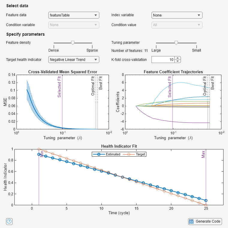
Figure Health Indicator Designer contains 3 axes objects and another object of type uigridlayout. Axes object 1 with title Health Indicator Fit, xlabel Time (cycle), ylabel Health Indicator contains 4 objects of type line, constantline. These objects represent Estimated, Target, Left, Right. Axes object 2 with title Feature Coefficient Trajectories, xlabel Tuning parameter (\lambda), ylabel Coefficients contains 16 objects of type line, constantline. These objects represent Vdclink_reduced_env_sigstats/ClearanceFactor, Vdclink_reduced_env_sigstats/CrestFactor, Vdclink_reduced_env_sigstats/ImpulseFactor, Vdclink_reduced_env_sigstats/Kurtosis, Vdclink_reduced_env_sigstats/Mean, Vdclink_reduced_env_sigstats/PeakValue, Vdclink_reduced_env_sigstats/RMS, Vdclink_reduced_env_sigstats/SINAD, Vdclink_reduced_env_sigstats/SNR, Vdclink_reduced_env_sigstats/ShapeFactor, Vdclink_reduced_env_sigstats/Skewness, Vdclink_reduced_env_sigstats/Std, Vdclink_reduced_env_sigstats/THD, Best Fit, Optimal Fit, Selected Fit. Axes object 3 with title Cross-Validated Mean Squared Error, xlabel Tuning parameter (\lambda), ylabel MSE contains 7 objects of type patch, line, constantline. These objects represent MSE-1SE, MSE+1SE, MSE, Best Fit, Optimal Fit, Selected Fit.

The default model uses 11 features. Using the data tips in the plot (not shown), the fit error at end of life is about 0.09. This error is enough to show up visibly in the Health Indicator Fit plot. Adjust Tuning Parameter to Optimal Fit to reduce the EOL error.

This model still uses 11 features, but the EOL prediction error is now about 0.017, or slightly less than 0.02, which meets the objective, but which requires that the model retain a large number of features.

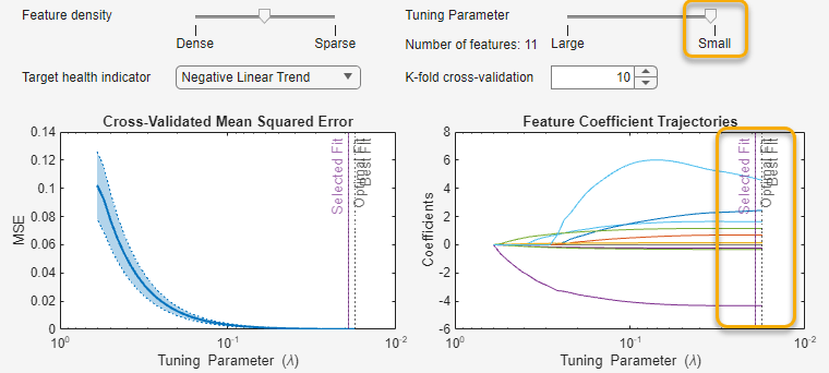
Move the tuning slider to the left until Number of features is 8.

The tuning error is now about 0.23, which does not meet the goal, and which visually deviates significantly from the target profile.

When you moved the tuning parameter, you excluded a number of features which appear to have similar trajectories, and which may be correlated. You can use the Feature density slider to include or exclude correlated features.

First, return λ to Optimal Fit. The Number of features returns to 11. Then, move the density slider to the right until Number of features drops to 8. Note that when you move the density slider, the app recalculates the grid of λ values. The position of Tuning parameter remains the same, but the corresponding value of λ changes to match the new grid location.

The EOL error is slightly under 0.02, about the same as it was for the 11-feature optimal fit.

Now move the density slider until Number of features is 7. The EOL error is still better than 0.02.

Move the density slider all the way to the right so that Number of features is 6.

The EOL error in this case is about 0.022, which exceeds the goal. The seven-feature model is the correct size for the HI.

An alternative way to reduce features while maintaining model accuracy is to use the Feature density slider first to get a sparser separation between features in the plot on the right and then fine-tune the Tuning parameter slider.

When you design a fused feature in Health Indicator Designer, you must make sure that the feature table rows are sorted in the same order as the progression of the system degradation, whether the feature table is compiled from multiple simulations or multiple files of measured data.

You can sort the feature rows within the feature table before you import it. Alternatively, you can append a sorting index to the feature table and use this index within the app.

Load the data, which includes the unsorted feature table featureTable_Presort and the index vector index.

load dclink_indexed featureTable_Presort index

Append index as the variable Index in the feature table.

featureTable_Indexed = featureTable_Presort;
featureTable_Indexed.Index = index;

Open the app using the indexed feature table.

healthIndicatorDesigner(featureTable_Indexed)

Figure Health Indicator Designer contains 3 axes objects and another object of type uigridlayout. Axes object 1 with title Health Indicator Fit, xlabel Time (cycle), ylabel Health Indicator contains 4 objects of type line, constantline. These objects represent Estimated, Target, Left, Right. Axes object 2 with title Feature Coefficient Trajectories, xlabel Tuning parameter (\lambda), ylabel Coefficients contains 17 objects of type line, constantline. These objects represent Vdclink_reduced_env_sigstats/ClearanceFactor, Vdclink_reduced_env_sigstats/CrestFactor, Vdclink_reduced_env_sigstats/ImpulseFactor, Vdclink_reduced_env_sigstats/Kurtosis, Vdclink_reduced_env_sigstats/Mean, Vdclink_reduced_env_sigstats/PeakValue, Vdclink_reduced_env_sigstats/RMS, Vdclink_reduced_env_sigstats/SINAD, Vdclink_reduced_env_sigstats/SNR, Vdclink_reduced_env_sigstats/ShapeFactor, Vdclink_reduced_env_sigstats/Skewness, Vdclink_reduced_env_sigstats/Std, Vdclink_reduced_env_sigstats/THD, Index, Best Fit, Optimal Fit, Selected Fit. Axes object 3 with title Cross-Validated Mean Squared Error, xlabel Tuning parameter (\lambda), ylabel MSE contains 7 objects of type patch, line, constantline. These objects represent MSE-1SE, MSE+1SE, MSE, Best Fit, Optimal Fit, Selected Fit.

When the app opens, by default, Index variable is set to None, so the features are not sorted, as the discontinuous appearance of the error and fit plots indicates.

The Index variable menu, however, contains all the variables in the feature table. Select Index.

The feature rows are sorted correctly.

Related Examples

Parameters

expand all

Select Data

Import a feature table to import from your MATLAB workspace by selecting the table variable name from the menu. The app recognizes feature tables in the form of tables, timetables, and numeric matrices, in which the columns or variables represent the features and condition variables, and the rows represent the ordered samples. If the samples are not ordered chronologically, use index to specify the ordering so that the features are consistent with the degradation profile.

You can combine the data from multiple feature profiles in a single feature column. For example, your table can combine feature data for three separate run-to-failure profiles. To combine them, your feature table must include the sample times.

  • For a timetable, specify sample times using with a rowTimes vector. Do not specify TimeStep when combining data from multiple sources.

  • For a table or matrix, include the sample times in a column vector, and specify the variable name of this column vector in index.

Select the name of a condition variable if you want to design an HI for a specific condition. The condition variable can represent, for example, an operating condition such as ambient temperature, or an identifier such as a specific machine or type of machine. Condition variable columns in a table or timetable must contain categorical, string, char array, or boolean values.

Select the condition value that corresponds with the condition variable. When you select a condition variable and a specific condition value, the app fuses a health indicator from only the features that match the condition. When you specify All, the app fuses the health indicator from all features regardless of the condition value.

Specify Parameters

Use the Feature density slider to tune the handling of correlated features. When this parameter is set to more dense, the app tends to retain all features that are cross-correlated. With a more sparse setting, for a set of correlated features, the app retains only the highest ranked features of the set. For a very sparse setting, the app either completely retains or completely discards a given set of correlated features. For more information about this parameter, see Algorithms.

The size of the tuning parameter λ influences the number of features that the HI incorporates. When λ is higher, the app fuses a smaller number of features at the expense of fit MSE. When λ is lower, the app fuses a larger number of features at the expense of variance and computational load. For more information about λ, see Algorithms.

The Number of Features value indicates the number of features in the model corresponding to the Selected Fit line in the Cross-Validated Mean Squared Error plot. The Feature density and Tuning Parameter settings both influence this number. You cannot set this parameter directly.

The target health indicator represents the degradation profile that you expect the RUL degradation to follow. As you vary the parameters of the app, your goal is to create a composite indicator that has a good fit to this target. The app includes profiles for a positive and a negative linear trend. Alternatively, you can assign one of your feature traces as a target.

You can also design a custom degradation profile, such as an exponential degradation profile, outside of the app. Then, append the data as a new variable in the feature table that you plan to import. After you import the feature table, assign Target health indicator to this new variable.

K-fold cross-validation uses data that has not been used to train the model to validate the model. This method partitions the data into subsets, or folds, and iteratively trains and tests models to determine the best performing model. This parameter is typically set to 5 or 10. Performing cross validation helps compute the error variance and can assist you in achieving your desired error performance with a smaller number of features.

Plots

This plot illustrates the mean squared error and the error variance of the fit of the current model with respect to the target profile.

  • The x-axis represents the tuning parameter λ, with a range that goes from high to low from left to right.

    • A higher value of λ corresponds to a lower number of features in the HI model and, therefore, a higher fit error.

    • A lower value of λ corresponds to a higher number of features and a lower fit error.

  • Three vertical lines represent the Selected Fit, Best Fit, and Optimal Fit positions of λ.

    • Selected Fit is the current value of λ in the model. You can drag this line interactively. Changing Selected Fit updates the HI model.

    • Best Fit is the value of λ that the software determines produces the best fit in terms of MSE.

    • Optimal Fit is the value of λ that the software determines to produce the best regularized fit in terms of both MSE and error variance.

This plot illustrates the changes in the coefficients of the HI linear regression solution as λ changes. A coefficient of 0 indicates that the solution does not include the corresponding feature. When λ is higher (toward the left side of the plot), the number of features tends to be lower and the coefficient values of the included features higher. When λ is lower, the number of features tends to be higher, and the coefficient values for more features start to rise as the model incorporates them. When multiple features show similar trajectories, they are likely to be correlated. Changing the Feature Density value removes or restores correlated trajectories in the plot.

This plot compares the value of the HI with the value of the target profile over the expected life duration.

Generate Code

Use Generate code to generate a MATLAB script that constructs the HI linear regression equation for the data sample passed in the input argument X. You can also use Generate code as you develop your HI to get insight into the current model.

The code includes the following information:

  • Selected condition variable and value (such as condition variable Machine with condition value Machine 1) in the feature table.

  • Selected rows (samples) and columns (features) in the feature table

  • Regression parameters, including the intercept (a0) in the regression equation) and the coefficients corresponding to the selected features

  • Value of the HI corresponding to X

Programmatic Use

expand all

healthIndicatorDesigner opens the Health Indicator Designer app.

healthIndicatorDesigner(featureTable) opens the Health Indicator Designer app and automatically loads the feature table featureTable.

Algorithms

Health Indicator Designer uses the elastic net method, which is related to the lasso algorithm (least absolute shrinkage and selection operator), from the Statistics and Machine Learning Toolbox™ to fit a model to the target. Elastic net regularization is a popular approach for model reduction, as it balances mean squared error and uncertainty.

The parameters and plots that the app displays are products of the lasso processing, which the app configures for the elastic net option. A key lasso tuning parameter is the regularization parameter λ, which influences how many predictors or, for Health Indicator Designer, features, to use in the model. The elastic net algorithm uses both λ and a second parameter, α, which, for elastic net, is constrained between 0 and 1. Using α has benefits especially when working with highly correlated predictors. In the app, the Feature density slider represents α.

For more information about the lasso and elastic net algorithms, see Lasso and Elastic Net.

References

[1] Zou, Hui, and Trevor Hastie. “Regularization and Variable Selection Via the Elastic Net.” Journal of the Royal Statistical Society Series B: Statistical Methodology, vol. 67, no. 2, Apr. 2005, pp. 301–20.

[2] Moradi, Morteza, et al. “Intelligent Health Indicator Construction for Prognostics of Composite Structures Utilizing a Semi-Supervised Deep Neural Network and SHM Data.” Engineering Applications of Artificial Intelligence, vol. 117, Jan. 2023, p. 105502. DOI.org (Crossref), https://doi.org/10.1016/j.engappai.2022.105502.

Version History

Introduced in R2024a