Diagnostic Feature Designer
Interactively extract, visualize, and rank features from measured or simulated data for machine diagnostics and prognostics
Description
The Diagnostic Feature Designer app allows you to accomplish the feature design portion of the predictive maintenance workflow using a multifunction graphical interface. You design and compare features interactively and then determine which features are best at discriminating between data from nominal systems and from faulty systems. The most effective features ultimately become your condition indicators for fault diagnosis and prognostics.
Using this app, you can:
Import measured or simulated data from individual files, an ensemble file, or an ensemble datastore that references files external to the app. You can also import data from Signal Labeler and Analog Input Recorder (Data Acquisition Toolbox), which can both export directly to Diagnostic Feature Designer, if you have the appropriate toolboxes installed and licensed.
Interactively visualize data to plot the ensemble variables you import or that you compute within the app. Group data by condition label in plots so that you can clearly see whether member data comes from nominal or faulty systems.
Derive new variables such as time-synchronous averaged signals or order spectra. The app executes processing on all ensemble members with one command.
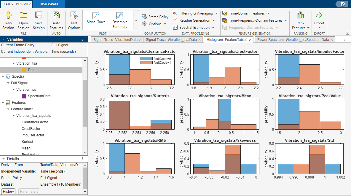
Generate features from your variables and visualize their effectiveness using histograms. Features include signal statistics, nonlinear metrics, rotating machinery metrics, and spectral metrics. You can also create your own custom features.
Rank your features to determine which ones are best at discriminating behavioral differences in the data.
Use supervised ranking with labeled features or system response data to determine which features are most likely to discriminate between nominal and faulty behavior.
Use unsupervised ranking when your data has no condition variables or labels to determine which features exhibit the best clustering with other features and are most likely to indicate different fault or operating conditions.
Use prognostic ranking with features extracted from run-to-failure data to determine which features are most likely to indicate remaining useful life (RUL).
Export your most effective features directly to Classification Learner or Regression Learner for more insight into feature effectiveness and for algorithm training.
Generate code for the features you choose so that you can reproduce, customize, and automate the feature computations in a MATLAB® function. You can also generate code and Simulink® blocks that support streaming data.
To get started with the app, you must have data from your systems available in your MATLAB workspace. For information about organizing your data for import into the app, see Organize System Data for Diagnostic Feature Designer.
For more information about condition indicators for predictive maintenance, see Condition Indicators for Monitoring, Fault Detection, and Prediction.
Open the Diagnostic Feature Designer App
MATLAB toolstrip: On the Apps tab, under Control System Design and Analysis, click the app icon.
MATLAB command prompt: Enter
diagnosticFeatureDesigner.
Examples
- Design Condition Indicators for Predictive Maintenance Algorithms
- Import and Visualize Ensemble Data in Diagnostic Feature Designer
- Process Data and Explore Features in Diagnostic Feature Designer
- Rank and Export Features in Diagnostic Feature Designer
- Broken Rotor Fault Detection in AC Induction Motors Using Vibration and Electrical Signals
- Prepare Matrix Data for Diagnostic Feature Designer
- Isolate a Shaft Fault Using Diagnostic Feature Designer
- Perform Prognostic Feature Ranking for a Degrading System Using Diagnostic Feature Designer
- Generate a MATLAB Function in Diagnostic Feature Designer
- Apply Generated MATLAB Function to Expanded Data Set
Parameters
Feature Designer Tab
Initiate a new app session by importing source data into the app from your MATLAB workspace. You can import data from tables, timetables, cell arrays, or matrices. You can import data from a single source that combines the data of multiple ensemble members or import individual ensemble members from separate sources. You can import labeled signal sets created in Signal Processing Toolbox™, as well as signals recorded using Analog Input Recorder (Data Acquisition Toolbox) in Data Acquisition Toolbox™. You can also import an ensemble datastore that contains information that allows the app to interact with external data files.
Your files can contain actual or simulated time-domain measurement data, spectral models or tables, variable names, condition and operational variables, and features you generated previously. Diagnostic Feature Designer combines all your member data into a single ensemble data set. In this data set, each variable is a collective signal or model that contains all the individual member values.
For more information about importing data, see Import Data into Diagnostic Feature Designer.
For more information about terms related to data ensembles, see More About.
For more information about organizing your data for import into the app, see Organize System Data for Diagnostic Feature Designer.
Generate and rank a feature set automatically using Auto Features. When you select one or more signals or spectra, Auto Features computes a predefined set of features that are appropriate for the variable type. You can choose from one or more feature sets:
Standard — Core features, including signal, spectral, and some time-frequency features
Advanced — Features that require more complex computations such as residual signals and detrended time series
Rotating Machinery — Specialized features for rotating machinery
The automatic computations include:
Deriving intermediate variables to use for feature extraction, such as spectra and time series signals
Extracting the features from the expanded variable set
Ranking the features and plotting the histograms of top-ranked features.
For more information, see Generate Features Automatically in Diagnostic Feature Designer.
Specify default plotting options for all plots that you generate during your app session. You can set these options before you generate your first plot, or at any time during your session. New settings apply only to plots that you generate after setting the options and not to plots that you generated earlier. You can temporarily override the Plot Options settings for individual plots without changing your specified defaults for subsequent plots. When you click Plot Options, you open a dialog box that allows you to set options in the following panes.
General — These options apply to all signal and spectrum plots.
Group by — Group data by a condition variable label. The app uses line thickness to distinguish label groups. For example, if your condition variable is
faultCodewith labelshealthyanddegraded, the app uses one thickness for member data with thehealthylabel and another thickness for member data with thedegradedlabel. To highlight the members of a specific label group, click the label in the plot legend.Number of curves — Specify the number of members to plot. Set this option when you have a large number of ensemble members and you want to plot only a subset of the members. Using this option reduces the plotting time and allows you to assess individual member behavior more easily.
Spectrum — These options apply only to spectral plots.
Number of peaks to mark — Specify the number of peaks to mark. Set this option to limit the number of spectral peaks that are marked to highlight only the most significant peaks.
Ensemble Summary — These options apply only to the ensemble summary plot, which is a special plot that displays the mean and standard deviation of the ensemble as a whole.
Number of standard deviations — Specify the number of standard deviations that the ensemble summary plot displays.
Show min and max boundaries — Specify whether to display the boundaries of the actual minimum and maximum values of the ensemble.
Generate a plot of an ensemble variable or feature table. To generate a plot, first select a variable or feature table from the Data Browser. The plot gallery shows icons for the compatible plot types. The following table describes the plot types for each type of selection.
| Input Type | Plot Type | Description | Customize With |
|---|---|---|---|
| Signal | Signal Trace | Ensemble signal data plotted by time or another independent variable that does not represent frequency. | Signal Trace Tab |
| Ensemble Summary | Mean, standard deviation, and min/max boundary for the ensemble as a whole. | Ensemble Summary Tab | |
| Spectrum | Power Spectrum | Ensemble signal power plotted by frequency. | Power Spectrum Tab |
| Order Spectrum | Ensemble signal power plotted by order, which is the ratio of a specific frequency to the main rotational frequency. | Order Spectrum Tab | |
| Feature Table | Histogram | Feature effectiveness, as visualized by a bar chart with color coding for the condition label. Effective features separate conditions cleanly. | |
| Feature Table View | Table containing feature values and their condition labels for each ensemble member. | N/A | |
| Feature Trace | Feature values for each member. This plot is especially useful for prognostic features (for RUL) computed from frame-based data. | Feature Selector |
Specify a frame policy when you want to perform data processing on sequential segments of a signal rather than the full signal at once. A frame policy consists of a frame size and a frame rate. The frame size is the interval over which the frame data is collected. The frame rate is the time interval between frame start times.
For more information on frame-based processing, see Data Handling Mode and Frame Policy.
Specify options when you want to modify one or both the following settings.
Select Independent Variable — Select the independent variable (IV) to use. When you import your data, you can specify more than one independent variable for a signal. For example, if your signal is time based, you might want to also have an independent variable for sample index. After you complete the import, you can change the independent variable that the app uses for a specific plot or computation. When you select Options > Select Independent Variable, the app displays a list of the available independent variables. Your selection changes the IV of all the applicable signals or spectra. For more information on specifying an alternate IV, see Specify Sample Index as Alternate IV in Import Data into Diagnostic Feature Designer.
Use Parallel Computing — Process ensemble members in parallel. Using parallel computing can significantly decrease processing time for large ensembles. This option is available only when you have Parallel Computing Toolbox™ installed and licensed.
Select options for processing your data into new signals or spectra. Use these new variables as inputs to other processing options or as inputs to feature generation. Most processing options operate on each ensemble member. You can also perform ensemble-level processing to view how the ensemble behaves as a whole. Each option selection opens a new tab for your specifications. Selection of an option also opens a general Data Processing tab if that tab is not already open. The Data Processing tab provides information about the input variable.
To specify a signal or spectrum to process, select a variable from the Variables pane prior to selecting the data processing option. To change the signal after opening the option tab, close the option tab and select a new signal either in the Variables pane or from the Signal list in the Data Processing tab.
You can perform the same processing on multiple variables at once by selecting multiple compatible variables (variables of the same type, such as signal or spectrum) in the Variables pane. You can also add additional variables after you select a processing operation. In the processing tab, select from the More Signals or More Spectra menu, which lists all the variables that are compatible with your initial variable selection.
Once you have configured your processing parameters, you can either
Execute the processing immediately (click Apply), or
Delay the execution and add it to a list containing multiple operations for later processing all at once (click Add Computation). The operations must be independent. You cannot, for example, compute a spectrum from a signal and then perform a frequency-domain operation on the new spectrum.
The Data Processing Computations panel records the name of the operation. When your processing list is complete, click Apply all.
A similar but separate computations list allows multiple-operation feature processing.
For more information about the processing options and the parameters that you can set for each option, see:
Filtering & Averaging
Residue Generation
Spectral Estimation
Select options for extracting features from your signals. Each option selection opens a new tab for your specifications. Selection of an option also opens a more general but category-specific features tab if that tab is not already open. This tab provides information about the input signal.
To specify a signal to extract features from, select a variable from the variables pane prior to selecting the feature option. To change the signal after opening the option tab, close the option tab and select a new signal either in the variables pane or from the Signal list in the feature tab.
Once you have configured your feature parameters, you can either
Execute the extraction immediately (click Apply), or
Delay the execution and add it to a list containing multiple operations for later processing all at once (click Add Computation).
The Feature Extraction Computations panel records the name of the operation. When your processing list is complete, click Apply all.
A similar but separate computations list allows multiple-operation data processing.
Compute features in the time domain. Signal Features apply to any signals. Time Series Features are features extracted from stationary time series. Model-based Features are features extracted using autoregressive (AR) models. Rotating Machinery Features are specialized metrics that apply to gearing. Nonlinear Features provide metrics that characterize chaotic behavior in vibration signals. Custom Features are features that you define by adding custom functions to the app. You can add existing MATLAB functions or create new functions using a template and then generate and rank the features alongside built-in app features
To specify a signal source for your features, select a signal variable from the variables pane prior to selecting the time-domain features option. To change the signal after opening the option tab, close the option tab and select a new signal either in the variables pane or from the Signal menu in the Time-Domain Features tab.
For more information about time-domain features options and the parameters that you can set for each option, see:
Time-Frequency features characterize signals whose frequencies change in time (that is, are nonstationary). Such signals can arise from machinery with degraded or failed hardware. The app provides two time-frequency feature options:
Spectrogram Features — Features based on spectrogram analysis. These features include:
Spectral Kurtosis metrics. The Spectral Kurtosis (SK) of a signal takes small values where only stationary Gaussian noise is present and high positive values at frequencies where transients occur. This capability makes SK a powerful tool for detecting and extracting signals associated with faults in rotating mechanical systems. The app can extract the features Crest Factor, Impulse Factor, Clearance Factor, and Peak Value from the SK signal. For more information on spectral kurtosis, and for information on setting Window Size, see
pkurtosis. For information on the SK signal metrics that the app extracts, see the corresponding definitions in Signal Features.Spectral Entropy. The spectral entropy (SE) of a signal is a measure of its spectral power distribution as it changes over time. Large changes in value can indicate faults. For more information spectral entropy, see
pentropy.
EMD Features — Features based on empirical mode decomposition (EMD). The empirical mode decomposition of a signal is a measure of the randomness of the unpredictability of the frequency content of a signal. An increase in the value can correspond to the presence of a fault. The app can extract the features Crest Factor, Impulse Factor, Clearance Factor, Peak Value, and Energy from the IMF signal that the EMD computation creates. For more information on empirical mode decomposition, and for information on setting Number of IMFs, see
emd. For information on the EMD metrics that the app extracts, see the corresponding definitions in Signal Features.
To specify a signal source for your features, select a signal variable from the variables pane prior to selecting the time-frequency-domain features option. To change the signal after opening the option tab, close the option tab and select a new signal either in the variables pane or from the Signal menu in the Time-Frequency-Domain Features tab.
Compute features in the frequency domain. Spectral Features are general metrics that apply to any spectrum, such as the peak amplitude across the full specified frequency range. Bearing Faults Features, Gear Mesh Faults Features, and Custom Faults Features are specialized metrics for rotating machinery that focus on spectral behavior within specific fault bands that bound characteristic frequencies, where faults can occur, of the components of the system. Custom Features are features that you define by adding custom functions to the app. You can add existing MATLAB functions or create new functions using a template and then generate and rank the features alongside built-in app features.
For more information about the frequency-domain features, see
Open the feature ranking tab to perform supervised, unsupervised, or prognostic ranking for the feature table that you select. For more information, see Feature Ranking Tab.
Export features, or your entire data set, to use them or share them outside of the app. Generate code to reproduce your feature computations in a MATLAB function or a Simulink block.
For feature export, both options open a list of features.
If you have not yet ranked your features, the app sorts this list by name, and marks all features by export by default. You can refine the selection if you want to export only specific features.
If you have ranked your features, the app sorts this list by your Sort by specification in the Feature Ranking Tab. Use Select top features to export only the most highly ranked features, based on the number of features that you specify. You can change the sorting order to alphabetical by selecting
Namein the Features sorted by list. With either sorting order, you can individually select or clear features to export.
When you export to the MATLAB workspace, you can use command-line techniques with the features. When you export to Classification Learner or Regression Learner, you open a new machine-learning session that uses your selected features as input.
For code generation, the first option,
Generate Function for
                  Features
, lets you generate MATLAB code with a simple set of specifications for feature table, ranking algorithm, and number of features. Use this option when you want to generate code for features based solely on ranking, or when you want to generate code for all your features.If you select Format for streaming data, the app generates a function that is compatible with MATLAB Coder™ and therefore supports streaming-data applications.
The second code generation option,
Generate Function
                  for...
, allows you to customize your selection of items to include in the function. For example, you can filter your selection based on criteria such as input or output text. You can include signals and spectra that are not used in the features you select. SelectingGenerate Function for...opens a selectable list of all the signals, features, and ranking tables that you have generated.Generate Function for...also opens the Code Generation tab, which provides filtering capability for the list. Use a filter to view only the items that meet the filter criterion. You can use different filters to select the outputs you want. To review all your selections regardless of filter, click Sort by Selection. This option lists all the available outputs with items that you selected on top. For more information, see Code Generation Tab.If you have specified frame-based data (see Options), clicking
Generate Function for...first opens a list with selections for the frame specifications that you have used. The items in your generated code must either all operate on the full signal or all use the same frame specification.The final option,
Generate Feature Extraction Simulink
                  Block
, exports a Simulink that incorporates the same streaming-formatted code that you generate inGenerate Function for Features.For more information on how to generate code or a Simulink in the app, see Automatic Feature Extraction Using Generated MATLAB Code, Generate a MATLAB Function in Diagnostic Feature Designer, and Export Feature Extraction Function and Simulink Model for Streaming Data.
For more information about the Export options, see:
Signal Trace, Ensemble Summary, Power Spectrum, and Order Spectrum Plot Tabs
Use the Panner to focus on data segments in the x-axis range that you specify and to change the plot scale. The Panner provides a strip plot beneath the main plot. To focus on a section of the main plot, move the handles. To change the scale of the plot, select one of the options in Scale.
Use the options in the first column of the View section to override the defaults in the Plot Options specification. The available options vary by plot type. For example, Number of Curves is an option for both signal traces and spectrum plots, while Number of Peaks to Mark is an option only for spectrum plots.
When you change these settings in the plot tab, you change them only for the current plot. For more information on these options, see Plot Options.
Use Normalize Y Axis when you are plotting multiple variables and want to view the variables on the same [-1, 1] scale. The relative signal amplitudes within a variable do not change.
In a signal or spectrum plot, you highlight an individual member by positioning your cursor on the member trace. Select Show Signal Information to display both the variable member that you highlight and the condition label for that member in the lower right corner.
If you select Data Cursors, Show Signal Information also displays the distance between the two cursors. For more information, see Data Cursors.
Specify how to plot multiple variables together.
Select to create a single plot that overlays all traces and uses a single y-axis scale.
Clear to create separate plots displayed vertically, each with a unique y-axis scaling.
Select Data Cursors to display values of key points in your signal. Data Cursors are horizontal and vertical bars that you position over a point of interest, such as a peak value. The cursors display the x and y positions. To display the distance between the cursors, select Show Signal Information. To lock the bars so that they move together, select one of the Lock Spacing options.
Histogram Tab
Click Select Features to open a selectable list of features to plot. Use Select Features, for example, when you have generated many features but you want to focus on a subset in a single plot panel.
For more information about selecting features, see Feature Selector.
Select the condition variable to base feature histograms on. The feature histograms use color to visualize the separation of data groups with different labels for that condition variable.
Example: faultCode
Specify histogram resolution using Bin Width, Binning Method, Number of Bins, and Bin Limits. The bin settings apply to all the histograms for the feature table.
The bin settings are not independent. The app histogram algorithm uses an order of precedence to determine what to use:
The Binning Method specification is the default driver for the bin width.
A Bin Width specification overrides the specified binning Method.
The bin width and the independent Bin Limits drive the number of bins. A Number of Bins specification has an effect only when the value of Group By is
none.The Normalization specification determines what the y axis represents. By default, the histograms use probability for the y axis, with a corresponding range from 0 to 1 for all features. Viewing multiple histograms on the same scale makes it easier to visually compare them. Choose other axis settings from the Normalization menu. These methods include raw counts and statistical metrics such as CDF.
For more information on interpreting and customizing histograms, see Generate and Customize Feature Histograms.
Feature Ranking Tab
Select a supervised ranking method to assess how effective each feature is for differentiating healthy behavior from unhealthy or degrading behavior. Diagnostic Feature Designer provides ranking methods for both classification and regression applications.
Classification ranking: Rank each feature on how well it separates data with different condition labels.
Regression ranking: Rank each feature on well it predicts numeric response data.
The menu includes two main sections — one for two-class and one for multiclass/regression ranking methods.
Two-Class Methods — Use a two-class method when your condition variable (CV) has only two labels, such as
“healthy”and“faulty”, or0and1. The default value for two-class methods isT-Test.Multiclass and Regression methods
Use a multiclass method when your condition variable has three or more labels, such as
“healthy”,“faultCode1”, and“faultCode2”, or0,1, and2. The default ranking for multiclass methods isOne-way ANOVA. You can also use multiclass methods for two-class applications.Use a regression method when your condition variable contains numeric response data. The default method is
MRMR. You can also use these regression ranking methods for classification ranking.
The app uses the CV content to determine which type of ranking – classification or regression - is likely to be applicable. However, for numeric data that could contain either condition labels or response values, you can change the ranking type in the tab.
The following table summarizes the ranking choices.
| Ranking Type* | Methods | Criteria | Links |
|---|---|---|---|
| Two-Class Classification | T-Test | Mean difference | ttest2 |
| Entropy | Relative entropy | relativeEntropy | |
| Bhattacharyya | Attainable classification error | bhattacharyyaDistance | |
| ROC | Area between ROC curve and random classifier slope | perfcurve | |
| Wilcoxon | Results of Wilcoxon test | ranksum | |
| Multiclass Classification | One-Way Anova | One-way analysis of variance | anova1 |
| Kruskal-Wallis | Chi-square statistic of Kruskal-Wallis test | kruskalwallis | |
| Regression | MRMR | Minimum Redundancy Maximum Relevance algorithm | fsrmrmr or fscmrmr |
| Relieff | Relieff (classification) or RRelieff (regression) algorithm | relieff | |
| *In this table, you can use the multiclass classification methods for two-class classification as well. Similarly, you can use the regression methods for either classification type. | |||
Selecting a method activates a new tab with a name that matches the ranking method. For more information on this method-activated tab, see Ranking Method Tabs.
If you have already ranked your features, you can rank them again with a different method and display the resulting rankings together.
Select an unsupervised classification ranking method to assess how effectively each feature performs when you do not have labeled data. The app provides two unsupervised ranking options:
Laplacian Score — Scores reflect how well features cluster with other features to form distinct groupings.
Variance — Scores reflect feature variance. Features with low variances tend to add less useful information to a model.
Selecting a method activates a new tab with a name that matches the ranking method. For more information on this tab, see Ranking Method Tabs.
For more information on the unsupervised ranking scoring, see:
Laplacian —
fsulaplacianVariance—
var
Unsupervised ranking is available in Diagnostic Feature Designer, but not in Classification Learner. If you plan to export your features to Classification Learner to train a model, you must use ensemble data that includes labels.
Select a prognostic ranking method to assess how effectively each feature tracks the degradation of your ensemble members when you have run-to-failure data. The top-ranking features are best at predicting the remaining useful life (RUL).
The app provides three prognostic ranking methods, all of which score features on a
scale ranging from 0 through 1. One method, Monotonicity, is
always available. The other two methods, Trendability and
Prognosability, are available only when you are using
frame-based data. The smaller data segments in frame-based data allow the tracking of
small changes that are induced by
degradation.
Monotonicity characterizes the trend of a feature as the system evolves toward failure. As a system gets progressively closer to failure, a suitable condition indicator has a monotonic positive or negative trend. For more information, see
monotonicity.Trendability provides a measure of similarity between the trajectories of a feature measured in multiple run-to-failure experiments. Trendability of a candidate condition indicator is defined as the smallest absolute correlation between measurements. For more information, see
trendability.Prognosability is a measure of the variability of a feature at failure relative to the range between its initial and final values. A more prognosable feature has less variation at failure relative to the range between its initial and final values. For more information, see
prognosability.
Selecting a method activates a new tab with a name that matches the ranking method. For more information on this method-activated tab, see Ranking Method Tab.
For an example of using prognostic ranking in the app, see Perform Prognostic Feature Ranking for a Degrading System Using Diagnostic Feature Designer.
Select the condition variable that provides the labels for the ranking algorithm to use.
Specify the ranking method to sort by when comparing the results of different ranking methods. When you use a single ranking method, the app displays the results in order of importance, as indicated by the ranking score for that method. When comparing the results for multiple methods, change Sort By to change the method that drives the sorting order.
Specify these parameters to perform one of the following deletion operations. The selection of Ranking method or Features below rank determines which operation the app performs.
Delete the scores from a ranking method — Select Ranking method to specify a ranking method to delete from the ranking table, and then, click Delete. Use this parameter, for example, when you compare the results of multiple rankings, and you want to simplify the display by eliminating rankings that do not influence your feature selection.
Delete low ranked features from the app — Select Features below rank to delete all features below the specified rank for the ranking method specified in Ranking method, and then, click Delete. For example, if you have 20 features and want to retain only the top five features according to the ranking method you specified, set Features below rank to 5. The app deletes the lowest 15 features.
To change the method on which the ranking is based, first, select Ranking Method and specify the method, and then, select Features below rank. Features below rank must be selected for Delete to delete features rather than remove a method.
Export features to use them or share them outside of the app. Generate code to reproduce your feature computations in a MATLAB function or a Simulink block.
Both options open a ranking-sorted selectable list to choose from. When you export to the MATLAB workspace, you can use command-line techniques with the features. When you export to the Classification Learner or Regression Learner, you open a machine-learning session that uses your selected features as input.
If you want to export your entire data set from the app, use Export from the Feature Designer tab.
You can also generate code or a Simulink block that reproduces the computations for the variables and features you
select. When you generate code using Generate Function for
Features from the Feature Ranking tab,
Ranking Method defaults to the method you specify in
Sort By. For more information about code generation, see the code
generation options description in the Export section in the
Feature Designer tab.
Ranking Method Tabs
The correlation importance setting allows you to screen out features that convey similar information to higher ranked features. This screening provides a more diverse feature set in the upper ranks.
The criterion for the screening is the set of cross-correlation coefficients a feature has with higher ranked features. High cross-correlation between two features implies that both features are separating condition groups similarly and provide redundant information. With the default value of 0, the app does not incorporate feature redundancy into ranking scores. As you increase the correlation importance value, the app increases the influence of feature cross-correlation on the feature ranking score. This increasing influence progressively lowers the score of redundant features.
The normalization scheme performs independent normalization across the members for every feature. Normalization allows more direct comparisons among features. The app displays the defining equation for the scheme you select directly beneath your selection.
This option is available only for supervised ranking and unsupervised Laplacian ranking methods.
Specify whether to rank features for classification or regression methods when the condition variable type (CV) is numeric. The app initializes the classification or regression selection based on the content of the CV, but you can switch that selection if it is not correct.
This option is available only for MRMR and Relieff ranking options.
Specify parameters that define key values for calculating the Laplacian score, which indicates how well a given feature clusters with other features. The Laplacian score is based on the pairwise distances from a given feature to its nearest neighbors.
Number of Neighbors — Number of nearest neighbors to use for computing the score
Distance Metric — Method, such as
euclideanorcityblock, for computing each pairwise distanceKernel Scale — Scale factor for the kernel that transforms the pairwise distances into a similarity graph that provides the scores
This option is available only for the unsupervised Laplacian ranking method. For
more information on Laplacian ranking, see fsulaplacian.
Click Apply to calculate a ranking with the specified parameters. The Feature Ranking tab in the plotting area displays the results both graphically and tabularly. This display also includes the results for the default ranking algorithm, and for any other ranking methods you calculated previously.
Once you calculate a ranking, the app disables Apply until you change a parameter. You can calculate a ranking within a tab multiple times. Each time you modify the parameters and calculate a ranking, the new results overwrite the previous results in the plotting-area tab.
Once you have completed your ranking within the ranking method tab, close that tab to return control to the Feature Ranking tab. The Feature Ranking is disabled while any ranking method tab is activated.
Code Generation Tab
This parameter is read-only.
The frame policy information reflects the choice you make when you select Export > Generate Function for... in the Feature Designer tab.
Set criteria to refine your options when selecting items for your generated function. All criteria allow you to overwrite selectable options with a string. String matching is case insensitive. Your filters apply to all output items, including signals, features, and ranking tables. Criteria include:
Output — String appearing in the output name, which is the name of the variable, feature, or ranking table to select for the generated function
Input — Input signal from which the output variable or feature was computed or feature table from which the ranking table was computed
Method — Computation that produced the output item, such as
TSAorKurtosisAnalysis Type — Data processing, feature processing, or feature ranking
To reset a single filter, delete the contents and click anywhere in the app. To reset all filters at once, click Reset Filters.
Display all selected items together. Use Sort Selected especially when you have used multiple filter combinations to assemble your codegen selections. All your selections appear together.
Specify whether to use parallel computing in the generated code. The default value is the value that is specified in Options. You can specify parallel computing even if you performed your interactive processing without using parallel computing. This approach helps your code to be more scalable if you plan to run the generated code on a larger ensemble than the ensemble you used to develop the features. You can also turn parallel computing off if you used it when you developed the features.
To take advantage of parallel processing in generated code, the user must have Parallel Computing Toolbox installed and licensed. However, the code will still run in serial mode on systems that do not have the toolbox.
Click the Generate Function button when you have completed configuring your selections. The app opens a function that contains computations used for all the output items you selected.
For more information about generating code in the app, see Automatic Feature Extraction Using Generated MATLAB Code.
Programmatic Use
diagnosticFeatureDesigner opens the Diagnostic Feature
Designer app.
diagnosticFeatureDesigner( opens
the app and loads a previously saved session. sessionFile)sessionFile is the name
of a session data file on the MATLAB path. The data includes all of the variables and features that you either
imported into the app or computed within the app. The data also includes your app settings
and the processing information necessary to generate code.
To save a session, in the Diagnostic Feature Designer app, on the
Feature Designer tab, click ![]() Save Session.
Save Session.
diagnosticFeatureDesigner( opens the
app and, after performing a validity check, automatically opens the New
Session dialog box with the data in dataset)dataset preselected as
the source.
More About
A data ensemble is a collection of data sets, created by measuring or simulating a system under varying conditions. An ensemble can be implemented using independent data sets such as matrices or tables, or in a single collective data set such as an ensemble table.
For more information on data ensembles and variables, see Data Ensembles for Condition Monitoring and Predictive Maintenance.
Each data set within an ensemble is a member. Members of an ensemble all contain the same variables. For example, if your ensemble contains data from a set of similar machines, the data set corresponding to one of those machines is a member.
An ensemble table is an ensemble data set formatted as a table. Each column of the table represents one variable. Each row of the table
represents one ensemble member. For information on converting member matrices to an ensemble
table, see Prepare Matrix Data for Diagnostic Feature Designer.
Large ensembles can be implemented using an ensemble datastore object. These objects contain a list of the member files and information for interacting with them. For more information on ensemble datastore objects, see Data Ensembles for Condition Monitoring and Predictive Maintenance.
Data variables make up the main content of the ensemble members,
including measured data and derived data that you use for analysis and development of
predictive maintenance algorithms. For example, you might represent accelerometer data as
the data variable Vibration. Data variables can also include derived
values, such as the mean value of a signal, or the frequency of the peak magnitude in a
signal spectrum.
Independent variables (IV) are the variables that identify or
order the members in an ensemble, such as timestamps, number of operating hours, or machine
identifiers. For example, Time is a common independent variable.
Condition variables (CV) are variables that describe the fault
condition or operating condition of the ensemble member. Condition variables can record the
presence or absence of a fault state, or other operating conditions such as ambient
temperature. Frequently condition variables have specific possible values described by
labels. For example, a condition variable named
Health might have two states described by labels
Healthy and Degraded. Condition variables can also
be derived values, such as a single scalar value that encodes multiple fault and operating
conditions.
Version History
Introduced in R2019a
See Also
Topics
- Explore Ensemble Data and Compare Features Using Diagnostic Feature Designer
- Organize System Data for Diagnostic Feature Designer
- Interpret Feature Histograms in Diagnostic Feature Designer
- Import Data into Diagnostic Feature Designer
- Automatic Feature Extraction Using Generated MATLAB Code
- Anatomy of App-Generated MATLAB Code
- Data Ensembles for Condition Monitoring and Predictive Maintenance
MATLAB Command
You clicked a link that corresponds to this MATLAB command:
Run the command by entering it in the MATLAB Command Window. Web browsers do not support MATLAB commands.
选择网站
选择网站以获取翻译的可用内容,以及查看当地活动和优惠。根据您的位置,我们建议您选择:。
您也可以从以下列表中选择网站:
如何获得最佳网站性能
选择中国网站(中文或英文)以获得最佳网站性能。其他 MathWorks 国家/地区网站并未针对您所在位置的访问进行优化。
美洲
- América Latina (Español)
- Canada (English)
- United States (English)
欧洲
- Belgium (English)
- Denmark (English)
- Deutschland (Deutsch)
- España (Español)
- Finland (English)
- France (Français)
- Ireland (English)
- Italia (Italiano)
- Luxembourg (English)
- Netherlands (English)
- Norway (English)
- Österreich (Deutsch)
- Portugal (English)
- Sweden (English)
- Switzerland
- United Kingdom (English)