pentropy

(To be removed) Spectral entropy of signal

pentropy will be removed in a future release. Use spectralEntropy instead. For more information, see Version History.

Syntax

se = pentropy(xt)

se = pentropy(x,sampx)

se = pentropy(p,fp,tp)

se = pentropy(___,Name=Value)

[se,t] = pentropy(___)

pentropy(___)

Description

se = pentropy(xt) returns the Spectral Entropy of single-variable, single-column timetable xt as the timetable se. pentropy computes the spectrogram of xt using the default options of pspectrum.

example

se = pentropy(x,sampx) returns the spectral entropy of vector x, sampled at rate or time interval sampx, as a vector.

example

se = pentropy(p,fp,tp) returns the spectral entropy using the power spectrogram p, along with spectrogram frequency and time vectors fp and tp.

Use this syntax when you want to customize the options for pspectrum, rather than accept the default pspectrum options that pentropy applies.

example

se = pentropy(___,Name=Value) specifies additional properties using name-value arguments. Options include instantaneous or whole-signal entropy, scaling by white noise entropy, frequency limits, and time limits. You can use Name=Value with any of the input arguments in previous syntaxes.

example

[se,t] = pentropy(___) returns the spectral entropy se along with the time vector or timetable t. If se is a timetable, then t is equal to the row times of timetable se. This syntax does not apply if Instantaneous is set to false.

example

pentropy(___) with no output arguments plots the spectral entropy against time. If Instantaneous is set to false, the function outputs the scalar value of the spectral entropy.

Examples

collapse all

Plot Spectral Entropy of Signal

Open Live Script

Plot the spectral entropy of a signal expressed as a timetable and as a time series.

Generate a random series with normal distribution (white noise).

xn = randn(1000,1);

Create time vector t and convert to duration vector tdur. Combine tdur and xn in a timetable.

fs = 10;
ts = 1/fs;
t = 0.1:ts:100;
tdur = seconds(t);
xt = timetable(tdur',xn);

Plot the spectral entropy of the timetable xt.

pentropy(xt)
title('Spectral Entropy of White Noise Signal Timetable')

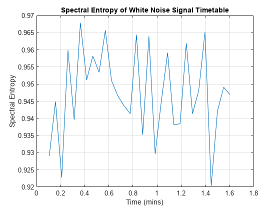
Figure contains an axes object. The axes object with title Spectral Entropy of White Noise Signal Timetable, xlabel Time (mins), ylabel Spectral Entropy contains an object of type line.

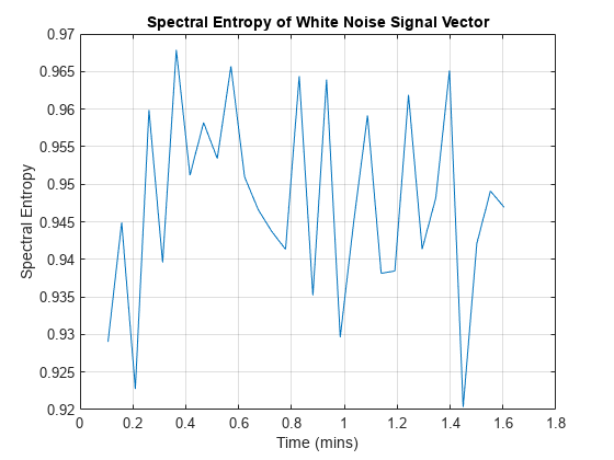
Plot the spectral entropy of the signal, using time-point vector t and the form which returns se and associated time te. Match the x-axis units and grid to the pentropy-generated plots for comparison.

[se,te] = pentropy(xn,t');
te_min = te/60;
plot(te_min,se)
title('Spectral Entropy of White Noise Signal Vector')
xlabel('Time (mins)')
ylabel('Spectral Entropy')
grid on

Figure contains an axes object. The axes object with title Spectral Entropy of White Noise Signal Vector, xlabel Time (mins), ylabel Spectral Entropy contains an object of type line.

Both yield the same result.

The second input argument for pentropy can represent either frequency or time. The software interprets according to the data type of the argument. Plot the spectral entropy of the signal, using sample rate scalar fs instead of time vector t.

pentropy(xn,fs)
title('Spectral Entropy of White Noise Signal Vector using Sample Rate')

Figure contains an axes object. The axes object with title Spectral Entropy of White Noise Signal Vector using Sample Rate, xlabel Time (mins), ylabel Spectral Entropy contains an object of type line.

This plot matches the previous plots.

Plot Spectral Entropy of Speech Signal

Open Live Script

Plot the spectral entropy of a speech signal and compare it to the original signal. Visualize the spectral entropy on a color map by first creating a power spectrogram, and then taking the spectral entropy of frequency bins within the bandwidth of speech.

Load the data x, which contains a two-channel recording of the word "Hello" embedded by low-level white noise. x consists of two columns representing the two channels. Use only the first channel.

Define the sample rate and the time vector. Augment the first channel of x with white noise to achieve a signal-to-noise ratio of about 5 to 1.

load Hello x
fs = 44100;
t = 1/fs*(0:length(x)-1);
x1 = x(:,1) + 0.01*randn(length(x),1);

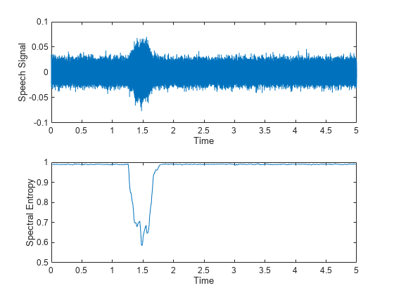
Find the spectral entropy. Visualize the data for the original signal and for the spectral entropy.

[se,te] = pentropy(x1,fs);

subplot(2,1,1)
plot(t,x1)
ylabel("Speech Signal")
xlabel("Time")

subplot(2,1,2)
plot(te,se)
ylabel("Spectral Entropy")
xlabel("Time")

Figure contains 2 axes objects. Axes object 1 with xlabel Time, ylabel Speech Signal contains an object of type line. Axes object 2 with xlabel Time, ylabel Spectral Entropy contains an object of type line.

The spectral entropy drops when "Hello" is spoken. This is because the signal spectrum has changed from almost a constant (white noise) to the distribution of a human voice. The human-voice distribution contains more information and has lower spectral entropy.

Compute the power spectrogram p of the original signal, returning frequency vector fp and time vector tp as well. For this case, specifying a frequency resolution of 20 Hz provides acceptable clarity in the result.

[p,fp,tp] = pspectrum(x1,fs,"spectrogram",...
    FrequencyResolution=20);

The frequency vector of the power spectrogram goes to 22,050 Hz, but the range of interest with respect to speech is limited to the telephony bandwidth of 300–3400 Hz. Divide the data into five frequency bins by defining start and end points, and compute the spectral entropy for each bin.

flow = [300 628 1064 1634 2394];
fup = [627 1060 1633 2393 3400];
 
se2 = zeros(length(flow),size(p,2));
for i = 1:length(flow)
    se2(i,:) = pentropy(p,fp,tp,...
        FrequencyLimits=[flow(i) fup(i)]);
end

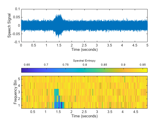
Visualize the data in a color map that shows ascending frequency bins, and compare with the original signal.

figure
tiledlayout flow
nexttile
plot(t,x1)
xlabel("Time (seconds)")
ylabel("Speech Signal")

nexttile
% Flip se2 so its plot corresponds 
% to the ascending frequency bins.
imagesc(tp,[],flip(se2))

h = colorbar(gca,"NorthOutside");
ylabel(h,"Spectral Entropy")
yticks(1:5)
set(gca,YTickLabel=num2str((5:-1:1).'))
xlabel("Time (seconds)")
ylabel("Frequency Bin")

Figure contains 2 axes objects. Axes object 1 with xlabel Time (seconds), ylabel Speech Signal contains an object of type line. Axes object 2 with xlabel Time (seconds), ylabel Frequency Bin contains an object of type image.

Use Spectral Entropy to Detect Sine Wave in White Noise

Open Live Script

Create a signal that combines white noise with a segment that consists of a sine wave. Use spectral entropy to detect the existence and position of the sine wave.

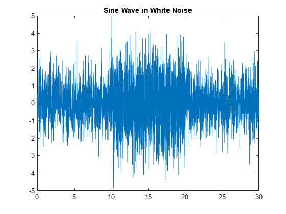
Generate and plot the signal, which contains three segments. The middle segment contains the sine wave along with white noise. The other two segments are pure white noise.

fs = 100;
t = 0:1/fs:10;
sin_wave = 2*sin(2*pi*20*t')+randn(length(t),1);
x = [randn(1000,1);sin_wave;randn(1000,1)];
t3 = 0:1/fs:30;

plot(t3,x)
title("Sine Wave in White Noise")

Figure contains an axes object. The axes object with title Sine Wave in White Noise contains an object of type line.

Plot the spectral entropy.

pentropy(x,fs)
title("Spectral Entropy of Sine Wave in White Noise")

Figure contains an axes object. The axes object with title Spectral Entropy of Sine Wave in White Noise, xlabel Time (secs), ylabel Spectral Entropy contains an object of type line.

The plot clearly differentiates the segment with the sine wave from the white-noise segments. This is because the sine wave contains information. Pure white noise has the highest spectral entropy.

The default for pentropy is to return or plot the instantaneous spectral entropy for each time point, as the previous plot displays. You can also distill the spectral entropy information into a single number that represents the entire signal by setting Instantaneous to false. Use the form that returns the spectral entropy value if you want to directly use the result in other calculations. Otherwise, pentropy returns the spectral entropy in ans.

se = pentropy(x,fs,Instantaneous=false)

se = 
0.9033

A single number characterizes the spectral entropy, and therefore the information content, of the signal. You can use this number to efficiently compare this signal with other signals.

Input Arguments

collapse all

`xt` — Signal timetable
timetable

Signal timetable from which pentropy returns the spectral entropy se, specified as a timetable that contains a single variable with a single column. xt must contain increasing, finite row times. If the xt timetable has missing or duplicate time points, you can fix it using the tips in Clean Timetable with Missing, Duplicate, or Nonuniform Times. xt can be nonuniformly sampled, with the pspectrum constraint that the median time interval and the mean time interval must obey:

$\frac{1}{100} < \frac{Median time interval}{Mean time interval} < 100.$

For an example, see Plot Spectral Entropy of Signal.

`x` — Time-series signal
vector

Time-series signal from which pentropy returns the spectral entropy se, specified as a vector.

`sampx` — Sample rate or sample time of signal
normalized frequency (default) | positive numeric scalar | `duration` scalar | numeric vector in seconds | `duration` array | `datetime` array

Sample rate or sample time, specified as one of the following:

Positive numeric scalar — Sample rate in hertz
duration scalar — Time interval between consecutive samples of X
Vector, duration array, or datetime array — Time instant or duration corresponding to each element of x

When sampx represents a time vector, time samples can be nonuniform, with the pspectrum constraint that the median time interval and the mean time interval must obey:

$\frac{1}{100} < \frac{Median time interval}{Mean time interval} < 100.$

For an example, see Plot Spectral Entropy of Signal.

`p` — Power spectrogram or spectrum of signal
real nonnegative matrix

Power spectrogram or spectrum of a signal, specified as a matrix (spectrogram) or a column vector (spectrum). If you specify p, then pentropy uses p rather than generate its own spectrogram or power spectrogram. fp and tp, which provide the frequency and time information, must accompany p. Each element of p at the i'th row and the j'th column represents the signal power at the frequency bin centered at fp(i) and the time instance tp(j).

For an example, see Plot Spectral Entropy of Speech Signal.

`fp` — Frequencies for spectrogram p
vector

Frequencies for spectrogram or power spectrogram p when p is supplied explicitly to pentropy, specified as a vector in hertz. The length of fp must be equal to the number of rows in s.

`tp` — Time information for spectrogram p
vector | `duration` array | `datetime` array

Time information for power spectrogram or spectrum p when p is supplied explicitly to pentropy, specified as one of the following:

Vector of time points, whose data type can be numeric, duration, or datetime. The length of vector tp must be equal to the number of columns in p.
duration scalar that represents the time interval in p. The scalar form of tp can be used only when p is a power spectrogram matrix.
For the special case where p is a column vector (power spectrum), tp can be a numeric, duration, or datetime scalar representing the time point of the spectrum.

For the special case where p is a column vector (power spectrum), tp can be a single/double/duration/datetime scalar representing the time point of the spectrum.

Name-Value Arguments

Specify optional pairs of arguments as Name1=Value1,...,NameN=ValueN, where Name is the argument name and Value is the corresponding value. Name-value arguments must appear after other arguments, but the order of the pairs does not matter.

Before R2021a, use commas to separate each name and value, and enclose Name in quotes.

Example: "Instantaneous",false,"FrequencyLimits",[25 50] computes the scalar spectral entropy representing the portion of the signal ranging from 25 Hz to 50 Hz.

`Instantaneous` — Instantaneous time series option
`true` (default) | `false`

Instantaneous time series option, specified as a logical.

If Instantaneous is true, then pentropy returns the instantaneous spectral entropy as a time-series vector.
If Instantaneous is false, then pentropy returns the spectral entropy value of the whole signal or spectrum as a scalar.

For an example, see Use Spectral Entropy to Detect Sine Wave in White Noise.

`Scaled` — Scale by white noise option
`true` (default) | `false`

Scale by white noise option, specified as a logical. Scaling by white noise — or log₂n, where n is the number of frequency points — is equivalent to normalizing in Spectral Entropy. It allows you to perform a direct comparison on signals of different length.

If Scaled is true, then pentropy returns the spectral entropy scaled by the spectral entropy of the corresponding white noise.
If Scaled is false, then pentropy does not scale the spectral entropy.

`FrequencyLimits` — Frequency limits
[0 `sampfreq`/2] (default) | [f1 f2]

Frequency limits to use, specified as a two-element vector containing lower and upper bounds f1 and f2 in hertz. The default is [0 sampfreq/2], where sampfreq is the sample rate in hertz that pentropy derives from sampx.

This specification allows you to exclude a band of data at either end of the spectral range.

For an example, see Plot Spectral Entropy of Speech Signal.

`TimeLimits` — Time Limits
full timespan (default) | [t1 t2]

Time limits, specified as a two-element vector containing lower and upper bounds t1 and t2 in the same units as the sample time provided in sampx, and of the data types:

Numeric or duration when sampx is numeric or duration
Numeric, duration, or datetime when sampx is datetime

This specification allows you to extract a time segment of data from the full timespan.

Output Arguments

collapse all

`se` — Spectral entropy
timetable | double vector

Spectral Entropy, returned as a timetable if the input signal is timetable xt, and as a double vector if the input signal is time series x.

`t` — time values corresponding to `se`
timetable | double vector

Time values associated with se, returned in the same form as the time in se. This argument does not apply if Instantaneous is set to false.

For an example, see Plot Spectral Entropy of Signal.

More About

collapse all

Spectral Entropy

The spectral entropy (SE) of a signal is a measure of its spectral power distribution. The concept is based on the Shannon entropy, or information entropy, in information theory. The SE treats the signal's normalized power distribution in the frequency domain as a probability distribution, and calculates the Shannon entropy of it. The Shannon entropy in this context is the spectral entropy of the signal. This property can be useful for feature extraction in fault detection and diagnosis. SE is also widely used as a feature in speech recognition and biomedical signal processing.

The equations for spectral entropy arise from the equations for the power spectrum and probability distribution for a signal. For a signal x(n), the power spectrum is S(m) = |X(m)|², where X(m) is the discrete Fourier transform of x(n). The probability distribution P(m) is then:

$P (m) = \frac{S (m)}{\sum_{i} S (i)} .$

The spectral entropy H follows as:

$H = - \sum_{m = 1}^{N} P (m) \log_{2} P (m) .$

Normalizing:

$H_{n} = - \frac{\sum_{m = 1}^{N} P (m) \log_{2} P (m)}{\log_{2} N},$

where N is the total frequency points. The denominator, log₂N represents the maximal spectral entropy of white noise, uniformly distributed in the frequency domain.

If a time-frequency power spectrogram S(t,f) is known, then the probability distribution becomes:

$P (m) = \frac{\sum_{t} S (t, m)}{\sum_{f} \sum_{t} S (t, f)} .$

Spectral entropy is still:

$H = - \sum_{m = 1}^{N} P (m) \log_{2} P (m) .$

To compute the instantaneous spectral entropy given a time-frequency power spectrogram S(t,f), the probability distribution at time t is:

$P (t, m) = \frac{S (t, m)}{\sum_{f} S (t, f)} .$

Then the spectral entropy at time t is:

$H (t) = - \sum_{m = 1}^{N} P (t, m) \log_{2} P (t, m) .$

References

[1] Pan, Y. N., J. Chen, and X. L. Li. "Spectral Entropy: A Complementary Index for Rolling Element Bearing Performance Degradation Assessment." Proceedings of the Institution of Mechanical Engineers, Part C: Journal of Mechanical Engineering Science. Vol. 223, Issue 5, 2009, pp. 1223–1231.

[2] Sharma, V., and A. Parey. "A Review of Gear Fault Diagnosis Using Various Condition Indicators." Procedia Engineering. Vol. 144, 2016, pp. 253–263.

[3] Shen, J., J. Hung, and L. Lee. "Robust Entropy-Based Endpoint Detection for Speech Recognition in Noisy Environments." ICSLP. Vol. 98, November 1998.

[4] Vakkuri, A., A. Yli‐Hankala, P. Talja, S. Mustola, H. Tolvanen‐Laakso, T. Sampson, and H. Viertiö‐Oja. "Time‐Frequency Balanced Spectral Entropy as a Measure of Anesthetic Drug Effect in Central Nervous System during Sevoflurane, Propofol, and Thiopental Anesthesia." Acta Anaesthesiologica Scandinavica. Vol. 48, Number 2, 2004, pp. 145–153.

Extended Capabilities

C/C++ Code Generation
Generate C and C++ code using MATLAB® Coder™.

Usage notes and limitations:

If the input signal is a timetable, the value of Instantaneous must be constant during code generation.

GPU Arrays
Accelerate code by running on a graphics processing unit (GPU) using Parallel Computing Toolbox™.

This function fully supports GPU arrays. For more information, see Run MATLAB Functions on a GPU (Parallel Computing Toolbox).

Version History

Introduced in R2018a

expand all

R2024b: `pentropy` will be removed

The pentropy function will be removed in a future release. Use spectralEntropy instead. You must update your code to use spectralEntropy.

Consider a signal x sampled at a rate fs:

fs = 1000;
Ts = seconds(1/fs);
t = (0:1/fs:10)';

x = chirp(t,300,10,400);
xT = timetable(x,SampleRate=fs);

To get the spectral entropy with spectralEntropy, make these updates to your code.

Original Code in R2024a or Earlier	Updated Code in R2024b
se = pentropy(xT);	[S,f,T] = pspectrum(xT,"spectrogram"); sE = timetable(T,spectralEntropy(S,f));
se = pentropy(x,fs);	[S,f] = pspectrum(x,fs,"spectrogram"); sE = spectralEntropy(S,f);
se = pentropy(x,Ts);	[S,f] = pspectrum(x,Ts,"spectrogram"); sE = spectralEntropy(S,f);
se = pentropy(x,t);	[S,f] = pspectrum(x,t,"spectrogram"); sE = spectralEntropy(S,f);
[S,f,T] = pspectrum(x,fs,"spectrogram"); se = pentropy(S,f,T);	[S,f] = pspectrum(x,fs,"spectrogram"); sE = spectralEntropy(S,f);
[S,f,T] = pspectrum(x,Ts,"spectrogram"); se = pentropy(S,f,T);	[S,f] = pspectrum(x,Ts,"spectrogram"); sE = spectralEntropy(S,f);
[S,f,T] = pspectrum(x,t,"spectrogram"); se = pentropy(S,f,T);	[S,f] = pspectrum(x,t,"spectrogram"); sE = spectralEntropy(S,f);

You can use the Scaled name-value argument in spectralEntropy just like in pentropy.
You can use the Instantaneous name-value argument in spectralEntropy just like in pentropy.
spectralEntropy does not support the FrequencyLimits name-value argument.
spectralEntropy does not support the TimeLimits name-value argument.

R2024a: Use timetables, datetime arrays and duration arrays for C/C++ code generation

The pentropy function supports MATLAB^® timetables, datetime arrays, and duration arrays for code generation. You must have MATLAB Coder™ to use this functionality.

pentropy

Syntax

Description

Examples

Plot Spectral Entropy of Signal

Plot Spectral Entropy of Speech Signal

Use Spectral Entropy to Detect Sine Wave in White Noise

Input Arguments

xt — Signal timetable timetable

x — Time-series signal vector

sampx — Sample rate or sample time of signal normalized frequency (default) | positive numeric scalar | duration scalar | numeric vector in seconds | duration array | datetime array

p — Power spectrogram or spectrum of signal real nonnegative matrix

fp — Frequencies for spectrogram p vector

tp — Time information for spectrogram p vector | duration array | datetime array

Name-Value Arguments

Instantaneous — Instantaneous time series option true (default) | false

Scaled — Scale by white noise option true (default) | false

FrequencyLimits — Frequency limits [0 sampfreq/2] (default) | [f1 f2]

TimeLimits — Time Limits full timespan (default) | [t1 t2]

Output Arguments

se — Spectral entropy timetable | double vector

t — time values corresponding to se timetable | double vector

More About

Spectral Entropy

References

Extended Capabilities

C/C++ Code Generation Generate C and C++ code using MATLAB® Coder™.

GPU Arrays Accelerate code by running on a graphics processing unit (GPU) using Parallel Computing Toolbox™.

Version History

R2024b: pentropy will be removed

R2024a: Use timetables, datetime arrays and duration arrays for C/C++ code generation

See Also

`xt` — Signal timetable
timetable

`x` — Time-series signal
vector

`sampx` — Sample rate or sample time of signal
normalized frequency (default) | positive numeric scalar | `duration` scalar | numeric vector in seconds | `duration` array | `datetime` array

`p` — Power spectrogram or spectrum of signal
real nonnegative matrix

`fp` — Frequencies for spectrogram p
vector

`tp` — Time information for spectrogram p
vector | `duration` array | `datetime` array

`Instantaneous` — Instantaneous time series option
`true` (default) | `false`

`Scaled` — Scale by white noise option
`true` (default) | `false`

`FrequencyLimits` — Frequency limits
[0 `sampfreq`/2] (default) | [f1 f2]

`TimeLimits` — Time Limits
full timespan (default) | [t1 t2]

`se` — Spectral entropy
timetable | double vector

`t` — time values corresponding to `se`
timetable | double vector

C/C++ Code Generation
Generate C and C++ code using MATLAB® Coder™.

GPU Arrays
Accelerate code by running on a graphics processing unit (GPU) using Parallel Computing Toolbox™.

R2024b: `pentropy` will be removed