kurtogram

Compute the kurtogram of a nonstationary signal. Compare different level settings for the kurtogram. Examine a kurtogram that uses normalized frequency. Use the kurtogram to provide filter settings that can be used to preprocess the signal to enhance transient detection.

Generate a signal with a chirp component and white Gaussian noise.

fs = 1000;
t = 0:1/fs:10;
f1 = 300;
f2 = 400;
xc = chirp(t,f1,10,f2);
x = xc+randn(1,length(t));

Plot the kurtogram using the sample rate fs.

kurtogram(x,fs)

The kurtogram shows kurtosis results for a range of window lengths and frequencies. A high kurtosis level corresponds to a high level of nonstationary or non-Gaussian behavior. The peak kurtosis is provided in the text at the top, along with the window length and center frequency associated with it. The bandwidth is a function of the window length.

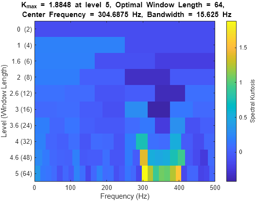
Explore the effects of lowering the maximum level to 5.

level = 5;
kurtogram(x,fs,level)

The lower resolution is apparent and leads to a lower peak kurtosis value and a displaced center frequency.

Now plot the kurtosis without specifying sample rate or time.

kurtogram(x)

The kurtogram is now shown with normalized frequency.

The parameters at the top of the plot provide recommendations for a bandpass filter that could be used to prefilter the data and enhance the differentiation of the nonstationary component. You can also have kurtogram return these values so they can be input more directly into filtering or spectral kurtosis functions.

[kgram,f,w,fc,wc,bw] = kurtogram(x);
wc

wc = 
256

fc

fc = 
2.4421

bw

bw = 
0.0245

These values match the optimal window size, center frequency, and bandwidth of the first plot. kgram is the actual kurtogram matrix, and f and w are the frequency and window-size vectors that accompany it.

The pkurtosis function uses the default pspectrum window size (time resolution). You can specify the window size to use instead. In this example, use the function kurtogram to return an optimal window size and use that result for pkurtosis.

Create a chirp signal with white Gaussian noise.

fs = 1000;
t = 0:1/fs:10;
f1 = 300;
f2 = 400;
x = chirp(t,f1,10,f2)+randn(1,length(t));

Plot the spectral kurtosis with the default window size.

pkurtosis(x,fs)
title('Spectral Kurtosis with Default Window Size')

Now compute the optimal window size using kurtogram.

kurtogram(x,fs)

The kurtogram plot also illustrates the chirp between 300 and 400 Hz, and shows that the optimum window size is 256. Feed w0 into pkurtosis.

w0 = 256;
pkurtosis(x,fs,w0)
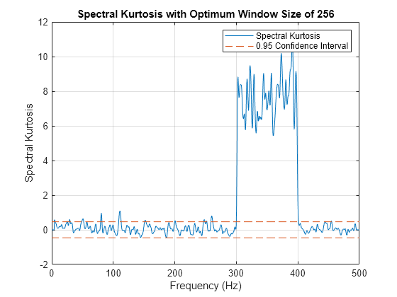
title('Spectral Kurtosis with Optimum Window Size of 256')

The main excursion has higher kurtosis values. The higher values improve the differentiation between stationary and nonstationary components, and enhance your ability to extract the nonstationary component as a feature.