pkurtosis

(To be removed) Spectral kurtosis from signal or spectrogram

pkurtosis will be removed in a future release. Use spectralKurtosis instead. For more information, see Version History.

Syntax

sk = pkurtosis(x)

sk = pkurtosis(x,sampx)

sk = pkurtosis(xt)

sk = pkurtosis(___,window)

sk = pkurtosis(s,sampx,f,window)

[sk,fout] = pkurtosis(___)

[___,thresh] = pkurtosis(___,'ConfidenceLevel',p)

pkurtosis(___)

Description

sk = pkurtosis(x) returns the spectral kurtosis of vector x as the vector sk. pkurtosis uses normalized frequency (evenly spaced frequency vector spanning [0 π]) to compute the time values. pkurtosis computes the spectrogram of x using pspectrum with default window size (time resolution in samples), and 80% window overlap.

example

sk = pkurtosis(x,sampx) returns the spectral kurtosis of vector x sampled at rate or time interval sampx.

example

sk = pkurtosis(xt) returns the spectral kurtosis of single-variable timetable xt in the vector sk. xt must contain increasing finite time samples.

sk = pkurtosis(___,window) returns the spectral kurtosis using the time resolution specified in window for the pspectrum spectrogram computation. You can use window with any of the input arguments in previous syntaxes.

example

sk = pkurtosis(s,sampx,f,window) returns the spectral kurtosis using the spectrogram or power spectrogram s, along with:

Sample rate or time, sampx, of the original time-series signal that was transformed to produce s
Spectrogram frequency vector f
Spectrogram time resolution window

Use this syntax when you want to customize the options for pspectrum, rather than accept the default pspectrum options that pkurtosis applies. You can specify sampx as empty to default to normalized frequency. Although window is optional for previous syntaxes, you must supply a value for window when using this syntax.

example

[sk,fout] = pkurtosis(___) returns the spectral kurtosis sk along with the frequency vector fout. You can use these output arguments with any of the input arguments in previous syntaxes.

[___,thresh] = pkurtosis(___,'ConfidenceLevel',p) returns the spectral kurtosis threshold thresh using the confidence level p. thresh represents the range within which the spectral kurtosis indicates a Gaussian stationary signal, at the optional confidence level p that you either specify or accept as default. Specifying p allows you to tune the sensitivity of the spectral kurtosis thresh results to behavior that is non-Gaussian or nonstationary. You can use the thresh output argument with any of the input arguments in previous syntaxes. You can also set the confidence level in previous syntaxes, but it has no effect unless you are returning or plotting thresh.

example

pkurtosis(___) plots the spectral kurtosis, along with confidence level and thresholds, without returning any data. You can use this syntax with any of the input arguments in previous syntaxes.

Examples

collapse all

Plot Spectral Kurtosis of Nonstationary Signal Using Different Confidence Levels

Open Live Script

Plot the spectral kurtosis of a chirp signal in white noise, and see how the nonstationary non-Gaussian regime can be detected. Explore the effects of changing the confidence level, and of invoking normalized frequency.

Create a chirp signal, add white Gaussian noise, and plot.

fs = 1000;
t = 0:1/fs:10;
f1 = 300;
f2 = 400;

xc = chirp(t,f1,10,f2);
x = xc + randn(1,length(t));

plot(t,x)
title('Chirp Signal with White Gaussian Noise')

Figure contains an axes object. The axes object with title Chirp Signal with White Gaussian Noise contains an object of type line.

Plot the spectral kurtosis of the signal.

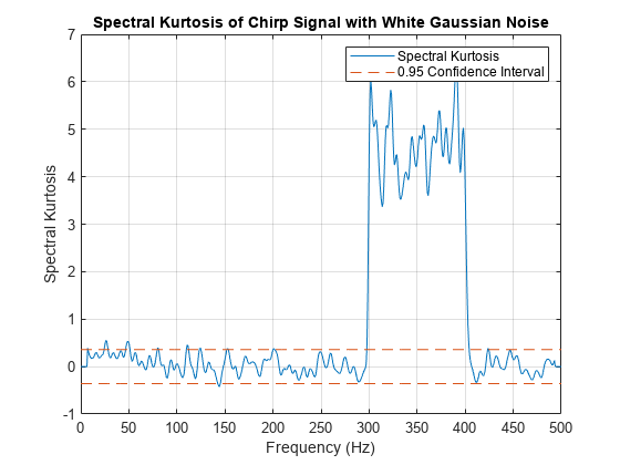
pkurtosis(x,fs)
title('Spectral Kurtosis of Chirp Signal with White Gaussian Noise')

Figure contains an axes object. The axes object with title Spectral Kurtosis of Chirp Signal with White Gaussian Noise, xlabel Frequency (Hz), ylabel Spectral Kurtosis contains 2 objects of type line. These objects represent Spectral Kurtosis, 0.95 Confidence Interval.

The plot shows a clear extended excursion from 300–400 Hz. This excursion corresponds to the signal component which represents the nonstationary chirp. The area between the two horizontal red-dashed lines represents the zone of probable stationary and Gaussian behavior, as defined by the 0.95 confidence interval. Any kurtosis points falling within this zone are likely to be stationary and Gaussian. Outside of the zone, kurtosis points are flagged as nonstationary or non-Gaussian. Below 300 Hz, there are a few additional excursions slightly above the above the zone threshold. These excursions represent false positives, where the signal is stationary and Gaussian, but because of the noise, has exceeded the threshold.

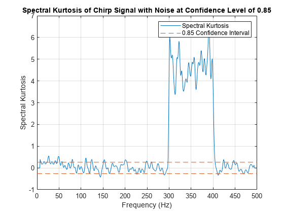
Investigate the impact of the confidence level by changing it from the default 0.95 to 0.85.

pkurtosis(x,fs,'ConfidenceLevel',0.85)
title('Spectral Kurtosis of Chirp Signal with Noise at Confidence Level of 0.85')

Figure contains an axes object. The axes object with title Spectral Kurtosis of Chirp Signal with Noise at Confidence Level of 0.85, xlabel Frequency (Hz), ylabel Spectral Kurtosis contains 2 objects of type line. These objects represent Spectral Kurtosis, 0.85 Confidence Interval.

The lower confidence level implies more sensitive detection of nonstationary or non-Gaussian frequency components. Reducing the confidence level shrinks the thresh-delimited zone. Now the low-level excursions — false alarms — have increased in both number and amount. Setting the confidence level is a balancing act between achieving effective detection and limiting the number of false positives.

You can accurately determine and compare the zone width for the two cases by using the pkurtosis form that returns it.

[sk1,~,thresh95] = pkurtosis(x);
[sk2,~,thresh85] = pkurtosis(x,'ConfidenceLevel',0.85);
thresh = [thresh95 thresh85]

thresh = 1×2

    0.3578    0.2628

Plot the spectral kurtosis again, but this time, omit the sample time information so that pkurtosis plots normalized frequency.

pkurtosis(x,'ConfidenceLevel',0.85)
title('Spectral Kurtosis using Normalized Frequency')

Figure contains an axes object. The axes object with title Spectral Kurtosis using Normalized Frequency, xlabel Normalized Frequency ( times blank pi blank radians/sample), ylabel Spectral Kurtosis contains 2 objects of type line. These objects represent Spectral Kurtosis, 0.85 Confidence Interval.

The frequency axis has changed from Hz to a scale from 0 to π rad/sample.

Plot Spectral Kurtosis Using a Customized Window Size

Open Live Script

The pkurtosis function uses the default pspectrum window size (time resolution). You can specify the window size to use instead. In this example, use the function kurtogram to return an optimal window size and use that result for pkurtosis.

Create a chirp signal with white Gaussian noise.

fs = 1000;
t = 0:1/fs:10;
f1 = 300;
f2 = 400;
x = chirp(t,f1,10,f2)+randn(1,length(t));

Plot the spectral kurtosis with the default window size.

pkurtosis(x,fs)
title('Spectral Kurtosis with Default Window Size')

Figure contains an axes object. The axes object with title Spectral Kurtosis with Default Window Size, xlabel Frequency (Hz), ylabel Spectral Kurtosis contains 2 objects of type line. These objects represent Spectral Kurtosis, 0.95 Confidence Interval.

Now compute the optimal window size using kurtogram.

kurtogram(x,fs)

Figure contains an axes object. The axes object with title K indexOf max baseline blank = blank 8 . 5267 blank at blank level blank 7 , blank Optimal blank Window blank Length blank = blank 256 , blank blank Center blank Frequency blank = blank 388 . 6719 blank Hz, blank Bandwidth blank = blank 3 . 9062 Hz, xlabel Frequency (Hz), ylabel Level (Window Length) contains an object of type image.

The kurtogram plot also illustrates the chirp between 300 and 400 Hz, and shows that the optimum window size is 256. Feed w0 into pkurtosis.

w0 = 256;
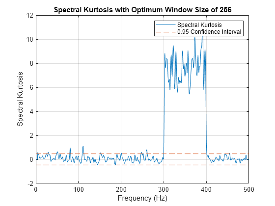
pkurtosis(x,fs,w0)
title('Spectral Kurtosis with Optimum Window Size of 256')

Figure contains an axes object. The axes object with title Spectral Kurtosis with Optimum Window Size of 256, xlabel Frequency (Hz), ylabel Spectral Kurtosis contains 2 objects of type line. These objects represent Spectral Kurtosis, 0.95 Confidence Interval.

The main excursion has higher kurtosis values. The higher values improve the differentiation between stationary and nonstationary components, and enhance your ability to extract the nonstationary component as a feature.

Plot Spectral Kurtosis Using a Customized Spectrogram

Open Live Script

When using signal input data, pkurtosis generates a spectrogram by using pspectrum with default options. You can also create the spectrogram yourself if you want to customize the options.

Create a chirp signal with white Gaussian noise.

fs = 1000;
t = 0:1/fs:10;
f1 = 300;
f2 = 400;
x = chirp(t,f1,10,f2)+randn(1,length(t));

Generate a spectrogram that uses your specification for window, overlap, and number of FFT points. Then use that spectrogram in pkurtosis.

window = 256;
overlap = round(window*0.8);
nfft = 2*window;
[s,f,t] = spectrogram(x,window,overlap,nfft,fs);
figure
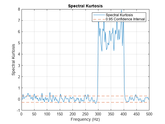
pkurtosis(s,fs,f,window)

Figure contains an axes object. The axes object with title Spectral Kurtosis, xlabel Frequency (Hz), ylabel Spectral Kurtosis contains 2 objects of type line. These objects represent Spectral Kurtosis, 0.95 Confidence Interval.

The magnitude of the excursion is higher, and therefore better differentiated, than with default inputs in previous examples. However, the excursion magnitude here is not as high as it is in the kurtogram-optimized window example.

Input Arguments

collapse all

`x` — Time-series signal
vector

Time-series signal from which pkurtosis returns the spectral kurtosis, specified as a vector.

`sampx` — Sample rate or sample time of signal
normalized frequency (default) | positive numeric scalar | `duration` scalar | numeric vector in seconds | `duration` array | `datetime` array

Sample rate or sample time, specified as one of the following::

Positive numeric scalar — frequency in hertz
duration scalar — time interval between consecutive samples of X
Vector, duration array, or datetime array — time instant or duration corresponding to each element of x

When sampx represents a time vector, time samples can be nonuniform, with the pspectrum constraint that the median time interval and the mean time interval must obey:

$\frac{1}{100} < \frac{Median time interval}{Mean time interval} < 100.$

If you specify sampx as empty, then pkurtosis uses normalized frequency. In other words, it assumes an evenly spaced frequency vector spanning [0 π].

`xt` — Signal timetable
timetable

Signal timetable from which pkurtosis returns the spectral kurtosis, specified as a timetable that contains a single variable with a single column. xt must contain increasing, finite row times. If the timetable has missing or duplicate time points, you can fix it using the tips in Clean Timetable with Missing, Duplicate, or Nonuniform Times. xt can be nonuniformly sampled, with the pspectrum constraint that the median time interval and the mean time interval must obey:

$\frac{1}{100} < \frac{Median time interval}{Mean time interval} < 100.$

`window` — Window time resolution
positive scalar

Window time resolution to use for the internal pspectrum spectrogram computation, specified as a positive scalar in samples. window is required for syntaxes that use an existing spectrogram as input, and optional for the rest. You can use the function kurtogram to determine the optimal window size to use. pspectrum uses 80% overlap by default.

`s` — Spectrogram or power spectrogram of signal
complex matrix | real nonnegative matrix

Power spectrogram or spectrum of a signal, specified as a matrix (spectrogram) or a column vector (spectrum).

If s is complex, then pkurtosis treats s as a short-time Fourier transform (STFT) of the original signal (spectrogram).
If s is real, then pkurtosis treats s as the square of the absolute values of the STFT of the original signal (power spectrogram). Thus, every element of s must be nonnegative.

If you specify s, pkurtosis uses s rather than generate its own spectrogram or power spectrogram. For an example, see Plot Spectral Kurtosis Using a Customized Spectrogram.

Data Types: single | double
Complex Number Support: Yes

`f` — Frequencies for s
vector

Frequencies for spectrogram or power spectrogram s when s is supplied explicitly to pkurtosis, specified as a vector in hertz. The length of f must be equal to the number of rows in s.

`'ConfidenceLevel'`, `p` — Confidence level
0.95 (default) | [0 to 1]

Confidence level used to determine whether signal is likely to be Gaussian and stationary, specified as a numeric scalar value from 0 to 1. p influences the thresh range where the spectral kurtosis value indicates a Gaussian and stationary signal. The confidence level therefore provides a detection-sensitivity tuning parameter. Kurtosis values outside of this range indicate, with a probability of (1-p), non-Gaussian or nonstationary behavior. For an example, see Plot Spectral Kurtosis of Nonstationary Signal Using Different Confidence Levels.

Output Arguments

collapse all

`sk` — Spectral kurtosis
double vector

Spectral Kurtosis, returned as a double vector. The spectral kurtosis is a statistical quantity that contains low values where data is stationary and Gaussian, and high values where transients occur. One use of the spectral kurtosis is to detect and locate nonstationary or non-Gaussian behavior that could result from faults or degradation. The high-valued kurtosis data reveals such signal components.

`fout` — frequencies for `sk`
double vector

Frequencies associated with sk values, returned as a vector in hertz.

`thresh` — Spectral kurtosis band size for stationary Gaussian behavior
scalar

Spectral kurtosis band size for stationary Gaussian behavior, returned as a numeric scalar representing the thickness of the band centered at the sk = 0 line, given confidence level p. Excursions outside the thresh-delimited band indicate possible nonstationary or non-Gaussian behavior. Confidence level p directly influences the thickness of the band and the sensitivity of the results. For an example, see Plot Spectral Kurtosis of Nonstationary Signal Using Different Confidence Levels.

More About

collapse all

Spectral Kurtosis

Spectral kurtosis (SK) is a statistical tool that can indicate and pinpoint nonstationary or non-Gaussian behavior in the frequency domain, by taking:

Small values at frequencies where only stationary Gaussian noise is present
High positive values at frequencies where transients occur

This capability makes SK a powerful tool for detecting and extracting signals associated with faults in rotating mechanical systems. On its own, SK can identify features or conditional indicators for fault detection and classification. As preprocessing for other tools such as envelope analysis, SK can supply key inputs such as optimal band [1], [2],.

The spectral kurtosis, or K(f), of a signal x(t) can be computed based on the short-time Fourier transform (STFT) of the signal, S(t,f):

$S (t, f) = \int_{- \infty}^{\infty} x (τ) w (τ - t) e^{- j 2 π f τ} d τ,$

where w(t) is the window function used in the STFT. K(f) is calculated as

$K (f) = \frac{{〈 {| S (t, f) |}^{4} 〉}_{t}}{{〈 {| S (t, f) |}^{2} 〉}_{t}^{2}} - 2, f \neq 0,$

where 〈·〉_t is the time-average operator.

If the signal x(t) contains only stationary Gaussian noise, then K(f) at each frequency f has an asymptotic normal distribution with 0 mean and variance 4/M, where M is the number of elements along the time axis in S(t,f). Hence, a statistical threshold s_α given a confidence level α is

$s_{α} = Φ^{- 1} (α) \frac{2}{\sqrt{M}},$

where $Φ^{- 1} (α) = \sqrt{2} \erf^{- 1} (2 α - 1)$ is the quantile function of the standard normal distribution.

It is important to note that the STFT window length N_w directly drives frequency resolution, which is f_s/N_w, where f_s is the sample rate. The window size must be shorter than the spacing between transient impulses but longer than the individual transient impulses.

References

[1] Antoni, J. "The Spectral Kurtosis: A Useful Tool for Characterising Non-Stationary Signals." Mechanical Systems and Signal Processing. Vol. 20, Issue 2, 2006, pp. 282–307.

[2] Antoni, J., and R. B. Randall. "The Spectral Kurtosis: Application to the Vibratory Surveillance and Diagnostics of Rotating Machines." Mechanical Systems and Signal Processing. Vol. 20, Issue 2, 2006, pp. 308–331.

Extended Capabilities

C/C++ Code Generation
Generate C and C++ code using MATLAB® Coder™.

GPU Arrays
Accelerate code by running on a graphics processing unit (GPU) using Parallel Computing Toolbox™.

The pkurtosis function supports GPU array input with these usage notes and limitations:

If the input is a pure tone signal, the result may show small numerical differences with respect to in-memory computation of spectral kurtosis.

For more information, see Run MATLAB Functions on a GPU (Parallel Computing Toolbox).

Version History

Introduced in R2018a

expand all

R2024b: `pkurtosis` will be removed

The pkurtosis function will be removed in a future release. Use spectralKurtosis instead. You must update your code to use spectralKurtosis.

Consider a signal x sampled at a rate fs:

fs = 1000;
Ts = seconds(1/fs);
t = (0:1/fs:10)';

x = chirp(t,300,10,400);
xT = timetable(x,SampleRate=fs);

function y = winlen(x)
    wdiv = 2.^[1 3:7];
    y = ceil(x/wdiv(find(x < 2.^[6 11:14 Inf],1)));
end

wnd = 500;

[Sstft,Fstft] = stft(x,fs, ...
    FrequencyRange="onesided", ...
    Window=triang(600),FFTLength=1512,OverlapLength=421);

To get the spectral kurtosis with spectralKurtosis, make these updates to your code..

Original Code in R2024a or Earlier	Updated Code in R2024b
sk = pkurtosis(xT);	[S,F] = pspectrum(xT,"spectrogram", ... FrequencyResolution= ... xT.Properties.SampleRate/winlen(height(xT)), ... OverlapPercent=80); sK = spectralKurtosis(S,F,Scaled=false);
sk = pkurtosis(x);	[S,F] = pspectrum(x,1,"spectrogram", ... FrequencyResolution= ... 1/winlen(length(x)), ... OverlapPercent=80); sK = spectralKurtosis(S,F,Scaled=false);
sk = pkurtosis(x,fs);	[S,F] = pspectrum(x,fs,"spectrogram", ... FrequencyResolution= ... fs/winlen(length(x)), ... OverlapPercent=80); sK = spectralKurtosis(S,F,Scaled=false);
sk = pkurtosis(x,Ts);	[S,F] = pspectrum(x,Ts,"spectrogram", ... FrequencyResolution= ... 1/(seconds(Ts)*winlen(length(x))), ... OverlapPercent=80); sK = spectralKurtosis(S,F,Scaled=false);
sk = pkurtosis(x,t);	[S,F] = pspectrum(x,t,"spectrogram", ... FrequencyResolution= ... 1/(mean(diff(t))*winlen(length(x))), ... OverlapPercent=80); sK = spectralKurtosis(S,F,Scaled=false);

sk = pkurtosis(xT,wnd);	[S,F] = pspectrum(xT,"spectrogram", ... FrequencyResolution= ... xT.Properties.SampleRate/wnd, ... OverlapPercent=80); sK = spectralKurtosis(S,F,Scaled=false);
sk = pkurtosis(x,[],wnd);	[S,F] = pspectrum(x,1,"spectrogram", ... FrequencyResolution=1/wnd, ... OverlapPercent=80); sK = spectralKurtosis(S,F,Scaled=false);
sk = pkurtosis(x,fs,wnd);	[S,F] = pspectrum(x,fs,"spectrogram", ... FrequencyResolution=fs/wnd, ... OverlapPercent=80); sK = spectralKurtosis(S,F,Scaled=false);
sk = pkurtosis(x,Ts,wnd);	[S,F] = pspectrum(x,Ts,"spectrogram", ... FrequencyResolution= ... 1/(seconds(Ts)*wnd), ... OverlapPercent=80); sK = spectralKurtosis(S,F,Scaled=false);
sk = pkurtosis(x,t,wnd);	[S,F] = pspectrum(x,t,"spectrogram", ... FrequencyResolution= ... 1/(mean(diff(t))*wnd), ... OverlapPercent=80); sK = spectralKurtosis(S,F,Scaled=false);

sk = pkurtosis(Sstft,fs,Fstft,wnd);	sK = spectralKurtosis(abs(Sstft).^2,Fstft, ... Scaled=false);
sk = pkurtosis(Sstft,fs,Fstft,wnd);	sK = spectralKurtosis(x,fs, ... Window=triang(600),FFTLength=1512, ... OverlapLength=421,Scaled=false);

You can use the ConfidenceLevel name-value argument in spectralKurtosis just like in pkurtosis.

R2023b: Use timetables for code generation

The pkurtosis function supports MATLAB^® timetables for code generation.

pkurtosis

Syntax

Description

Examples

Plot Spectral Kurtosis of Nonstationary Signal Using Different Confidence Levels

Plot Spectral Kurtosis Using a Customized Window Size

Plot Spectral Kurtosis Using a Customized Spectrogram

Input Arguments

`x` — Time-series signal
vector

`sampx` — Sample rate or sample time of signal
normalized frequency (default) | positive numeric scalar | `duration` scalar | numeric vector in seconds | `duration` array | `datetime` array

`xt` — Signal timetable
timetable

`window` — Window time resolution
positive scalar

`s` — Spectrogram or power spectrogram of signal
complex matrix | real nonnegative matrix

`f` — Frequencies for s
vector

`'ConfidenceLevel'`, `p` — Confidence level
0.95 (default) | [0 to 1]

Output Arguments

`sk` — Spectral kurtosis
double vector

`fout` — frequencies for `sk`
double vector

`thresh` — Spectral kurtosis band size for stationary Gaussian behavior
scalar

More About

Spectral Kurtosis

References

Extended Capabilities

C/C++ Code Generation
Generate C and C++ code using MATLAB® Coder™.

GPU Arrays
Accelerate code by running on a graphics processing unit (GPU) using Parallel Computing Toolbox™.

Version History

R2024b: `pkurtosis` will be removed

R2023b: Use timetables for code generation

See Also

Topics

pkurtosis

Syntax

Description

Examples

Plot Spectral Kurtosis of Nonstationary Signal Using Different Confidence Levels

Plot Spectral Kurtosis Using a Customized Window Size

Plot Spectral Kurtosis Using a Customized Spectrogram

Input Arguments

x — Time-series signal vector

sampx — Sample rate or sample time of signal normalized frequency (default) | positive numeric scalar | duration scalar | numeric vector in seconds | duration array | datetime array

xt — Signal timetable timetable

window — Window time resolution positive scalar

s — Spectrogram or power spectrogram of signal complex matrix | real nonnegative matrix

f — Frequencies for s vector

'ConfidenceLevel', p — Confidence level 0.95 (default) | [0 to 1]

Output Arguments

sk — Spectral kurtosis double vector

fout — frequencies for sk double vector

thresh — Spectral kurtosis band size for stationary Gaussian behavior scalar

More About

Spectral Kurtosis

References

Extended Capabilities

C/C++ Code Generation Generate C and C++ code using MATLAB® Coder™.

GPU Arrays Accelerate code by running on a graphics processing unit (GPU) using Parallel Computing Toolbox™.

Version History

R2024b: pkurtosis will be removed

R2023b: Use timetables for code generation

See Also

Topics

`x` — Time-series signal
vector

`sampx` — Sample rate or sample time of signal
normalized frequency (default) | positive numeric scalar | `duration` scalar | numeric vector in seconds | `duration` array | `datetime` array

`xt` — Signal timetable
timetable

`window` — Window time resolution
positive scalar

`s` — Spectrogram or power spectrogram of signal
complex matrix | real nonnegative matrix

`f` — Frequencies for s
vector

`'ConfidenceLevel'`, `p` — Confidence level
0.95 (default) | [0 to 1]

`sk` — Spectral kurtosis
double vector

`fout` — frequencies for `sk`
double vector

`thresh` — Spectral kurtosis band size for stationary Gaussian behavior
scalar

C/C++ Code Generation
Generate C and C++ code using MATLAB® Coder™.

GPU Arrays
Accelerate code by running on a graphics processing unit (GPU) using Parallel Computing Toolbox™.

R2024b: `pkurtosis` will be removed