Rolling Element Bearing Fault Diagnosis

Open Live Script

This example shows how to perform fault diagnosis of a rolling element bearing based on acceleration signals, especially in the presence of strong masking signals from other machine components. The example will demonstrate how to apply envelope spectrum analysis and spectral kurtosis to diagnose bearing faults and it is able to scale up to Big Data applications.

Problem Overview

Localized faults in a rolling element bearing may occur in the outer race, the inner race, the cage, or a rolling element. High frequency resonances between the bearing and the response transducer are excited when the rolling elements strike a local fault on the outer or inner race, or a fault on a rolling element strikes the outer or inner race [1]. The following picture shows a rolling element striking a local fault at the inner race. The problem is how to detect and identify the various types of faults.

Machinery Failure Prevention Technology (MFPT) Challenge Data

MFPT Challenge data [4] contains 23 data sets collected from machines under various fault conditions. The first 20 data sets are collected from a bearing test rig, with 3 under good conditions, 3 with outer race faults under constant load, 7 with outer race faults under various loads, and 7 with inner race faults under various loads. The remaining 3 data sets are from real-world machines: an oil pump bearing, an intermediate speed bearing, and a planet bearing. The fault locations are unknown. In this example, only the data collected from the test rig with known conditions are used.

Each data set contains an acceleration signal "gs", sampling rate "sr", shaft speed "rate", load weight "load", and four critical frequencies representing different fault locations: ballpass frequency outer race (BPFO), ballpass frequency inner race (BPFI), fundamental train frequency (FTF), and ball spin frequency (BSF). Here are the formulae for those critical frequencies [1].

Ballpass frequency, outer race (BPFO)

$B P F O = \frac{n f_{r}}{2} (1 - \frac{d}{D} \cos ϕ)$

Ballpass frequency, inner race (BPFI)

$B P F I = \frac{n f_{r}}{2} (1 + \frac{d}{D} \cos ϕ)$

Fundamental train frequency (FTF), also known as cage speed

$F T F = \frac{f_{r}}{2} (1 - \frac{d}{D} \cos ϕ)$

Ball (roller) spin frequency

$B S F = \frac{D f_{r}}{2 d} [1 - {(\frac{d}{D} \cos ϕ)}^{2}]$

As shown in the figure, $d$ is the ball diameter, $D$ is the pitch diameter. The variable $f_{r}$ is the shaft speed, $n$ is the number of rolling elements, $ϕ$ is the bearing contact angle [1].

Envelope Spectrum Analysis for Bearing Diagnosis

In the MFPT data set, the shaft speed is constant, hence there is no need to perform order tracking as a pre-processing step to remove the effect of shaft speed variations.

When rolling elements hit the local faults at outer or inner races, or when faults on the rolling element hit the outer or inner races, the impact will modulate the corresponding critical frequencies, e.g. BPFO, BPFI, FTF, BSF. Therefore, the envelope signal produced by amplitude demodulation conveys more diagnostic information that is not available from spectrum analysis of the raw signal. Take an inner race fault signal in the MFPT dataset as an example.

dataInner = load(fullfile(matlabroot, 'toolbox', 'predmaint', ...
    'predmaintdemos', 'bearingFaultDiagnosis', ...
    'train_data', 'InnerRaceFault_vload_1.mat'));

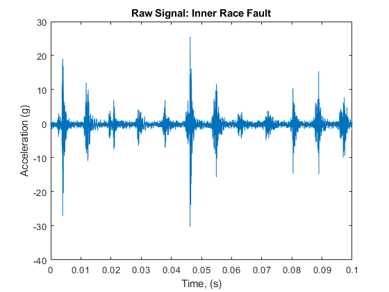
Visualize the raw inner race fault data in the time domain.

xInner = dataInner.bearing.gs;
fsInner = dataInner.bearing.sr;
tInner = (0:length(xInner)-1)/fsInner;
figure
plot(tInner, xInner)
xlabel('Time, (s)')
ylabel('Acceleration (g)')
title('Raw Signal: Inner Race Fault')
xlim([0 0.1])

Visualize the raw data in frequency domain.

figure
[pInner, fpInner] = pspectrum(xInner, fsInner);
pInner = 10*log10(pInner);
plot(fpInner, pInner)
xlabel('Frequency (Hz)')
ylabel('Power Spectrum (dB)')
title('Raw Signal: Inner Race Fault')
legend('Power Spectrum')

Now zoom in the power spectrum of the raw signal in low frequency range to take a closer look at the frequency response at BPFI and its first several harmonics.

figure
plot(fpInner, pInner)
ncomb = 10;
helperPlotCombs(ncomb, dataInner.BPFI)
xlabel('Frequency (Hz)')
ylabel('Power Spectrum (dB)')
title('Raw Signal: Inner Race Fault')
legend('Power Spectrum', 'BPFI Harmonics')
xlim([0 1000])

No clear pattern is visible at BPFI and its harmonics. Frequency analysis on the raw signal does not provide useful diagnosis information.

Looking at the time-domain data, it is observed that the amplitude of the raw signal is modulated at a certain frequency, and the main frequency of the modulation is around 1/0.009 Hz $\approx$ 111 Hz. It is known that the frequency the rolling element hitting a local fault at the inner race, that is BPFI, is 118.875 Hz. This indicates that the bearing potentially has an inner race fault.

figure
subplot(2, 1, 1)
plot(tInner, xInner)
xlim([0.04 0.06])
title('Raw Signal: Inner Race Fault')
ylabel('Acceleration (g)')
annotation('doublearrow', [0.37 0.71], [0.8 0.8])
text(0.047, 20, ['0.009 sec \approx 1/BPFI, BPFI = ' num2str(dataInner.BPFI)])

To extract the modulated amplitude, compute the envelope of the raw signal, and visualize it on the bottom subplot.

subplot(2, 1, 2)
[pEnvInner, fEnvInner, xEnvInner, tEnvInner] = envspectrum(xInner, fsInner);
plot(tEnvInner, xEnvInner)
xlim([0.04 0.06])
xlabel('Time (s)')
ylabel('Acceleration (g)')
title('Envelope signal')

Now compute the power spectrum of the envelope signal and take a look at the frequency response at BPFI and its harmonics.

figure
plot(fEnvInner, pEnvInner)
xlim([0 1000])
ncomb = 10;
helperPlotCombs(ncomb, dataInner.BPFI)
xlabel('Frequency (Hz)')
ylabel('Peak Amplitude')
title('Envelope Spectrum: Inner Race Fault')
legend('Envelope Spectrum', 'BPFI Harmonics')

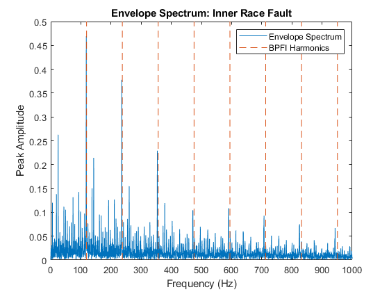
It is shown that most of the energy is focused at BPFI and its harmonics. That indicates an inner race fault of the bearing, which matches the fault type of the data.

Applying Envelope Spectrum Analysis to Other Fault Types

Now repeat the same envelope spectrum analysis on normal data and outer race fault data.

dataNormal = load(fullfile(matlabroot, 'toolbox', 'predmaint', ...
    'predmaintdemos', 'bearingFaultDiagnosis', ...
    'train_data', 'baseline_1.mat'));
xNormal = dataNormal.bearing.gs;
fsNormal = dataNormal.bearing.sr;
tNormal = (0:length(xNormal)-1)/fsNormal;
[pEnvNormal, fEnvNormal] = envspectrum(xNormal, fsNormal);

figure
plot(fEnvNormal, pEnvNormal)
ncomb = 10;
helperPlotCombs(ncomb, [dataNormal.BPFO dataNormal.BPFI])
xlim([0 1000])
xlabel('Frequency (Hz)')
ylabel('Peak Amplitude')
title('Envelope Spectrum: Normal')
legend('Envelope Spectrum', 'BPFO Harmonics', 'BPFI Harmonics')

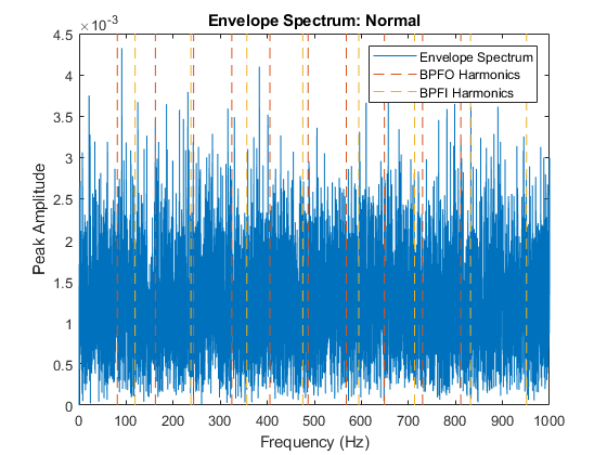
As expected, the envelope spectrum of a normal bearing signal does not show any significant peaks at BPFO or BPFI.

dataOuter = load(fullfile(matlabroot, 'toolbox', 'predmaint', ...
    'predmaintdemos', 'bearingFaultDiagnosis', ...
    'train_data', 'OuterRaceFault_2.mat'));
xOuter = dataOuter.bearing.gs;
fsOuter = dataOuter.bearing.sr;
tOuter = (0:length(xOuter)-1)/fsOuter;
[pEnvOuter, fEnvOuter, xEnvOuter, tEnvOuter] = envspectrum(xOuter, fsOuter);

figure
plot(fEnvOuter, pEnvOuter)
ncomb = 10;
helperPlotCombs(ncomb, dataOuter.BPFO)
xlim([0 1000])
xlabel('Frequency (Hz)')
ylabel('Peak Amplitude')
title('Envelope Spectrum: Outer Race Fault')
legend('Envelope Spectrum', 'BPFO Harmonics')

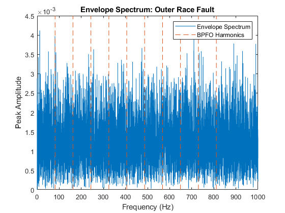
For an outer race fault signal, there are no clear peaks at BPFO harmonics either. Does envelope spectrum analysis fail to differentiate bearing with outer race fault from healthy bearings? Let's take a step back and look at the signals in time domain under different conditions again.

First let's visualize the signals in time domain again and calculate their kurtosis. Kurtosis is the fourth standardized moment of a random variable. It characterizes the impulsiveness of the signal or the heaviness of the random variable's tail.

figure
subplot(3, 1, 1)
kurtInner = kurtosis(xInner);
plot(tInner, xInner)
ylabel('Acceleration (g)')
title(['Inner Race Fault, kurtosis = ' num2str(kurtInner)])
xlim([0 0.1])

subplot(3, 1, 2)
kurtNormal = kurtosis(xNormal);
plot(tNormal, xNormal)
ylabel('Acceleration (g)')
title(['Normal, kurtosis = ' num2str(kurtNormal)])
xlim([0 0.1])

subplot(3, 1, 3)
kurtOuter = kurtosis(xOuter);
plot(tOuter, xOuter)
xlabel('Time (s)')
ylabel('Acceleration (g)')
title(['Outer Race Fault, kurtosis = ' num2str(kurtOuter)])
xlim([0 0.1])

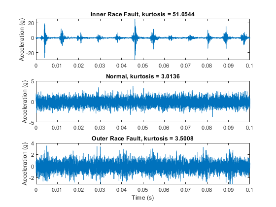
It is shown that inner race fault signal has significantly larger impulsiveness, making envelope spectrum analysis capture the fault signature at BPFI effectively. For an outer race fault signal, the amplitude modulation at BPFO is slightly noticeable, but it is masked by strong noise. The normal signal does not show any amplitude modulation. Extracting the impulsive signal with amplitude modulation at BPFO (or enhancing the signal-to-noise ratio) is a key preprocessing step before envelope spectrum analysis. The next section will introduce kurtogram and spectral kurtosis to extract the signal with highest kurtosis, and perform envelope spectrum analysis on the filtered signal.

Kurtogram and Spectral Kurtosis for Band Selection

Kurtogram and spectral kurtosis compute kurtosis locally within frequency bands. They are powerful tools to locate the frequency band that has the highest kurtosis (or the highest signal-to-noise ratio) [2]. After pinpointing the frequency band with the highest kurtosis, a bandpass filter can be applied to the raw signal to obtain a more impulsive signal for envelope spectrum analysis.

level = 9;
figure
kurtogram(xOuter, fsOuter, level)

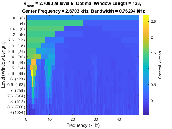
The kurtogram indicates that the frequency band centered at 2.67 kHz with a 0.763 kHz bandwidth has the highest kurtosis of 2.71.

Now use the optimal window length suggested by the kurtogram to compute the spectral kurtosis.

figure
wc = 128;
pkurtosis(xOuter, fsOuter, wc)

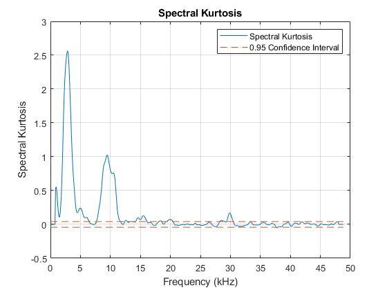
To visualize the frequency band on a spectrogram, compute the spectrogram and place the spectral kurtosis on the side. To interpret the spectral kurtosis in another way, high spectral kurtosis values indicates high variance of power at the corresponding frequency, which makes spectral kurtosis a useful tool to locate nonstationary components of the signal [3].

helperSpectrogramAndSpectralKurtosis(xOuter, fsOuter, level)

By bandpass filtering the signal with the suggested center frequency and bandwidth, the kurtosis can be enhanced and the modulated amplitude of the outer race fault can be retrieved.

[~, ~, ~, fc, ~, BW] = kurtogram(xOuter, fsOuter, level);

bpf = designfilt('bandpassfir', 'FilterOrder', 200, 'CutoffFrequency1', fc-BW/2, ...
    'CutoffFrequency2', fc+BW/2, 'SampleRate', fsOuter);
xOuterBpf = filter(bpf, xOuter);
[pEnvOuterBpf, fEnvOuterBpf, xEnvOuterBpf, tEnvBpfOuter] = envspectrum(xOuter, fsOuter, ...
    'FilterOrder', 200, 'Band', [fc-BW/2 fc+BW/2]);

figure
subplot(2, 1, 1)
plot(tOuter, xOuter, tEnvOuter, xEnvOuter)
ylabel('Acceleration (g)')
title(['Raw Signal: Outer Race Fault, kurtosis = ', num2str(kurtOuter)])
xlim([0 0.1])
legend('Signal', 'Envelope')

subplot(2, 1, 2)
kurtOuterBpf = kurtosis(xOuterBpf);
plot(tOuter, xOuterBpf, tEnvBpfOuter, xEnvOuterBpf)
ylabel('Acceleration (g)')
xlim([0 0.1])
xlabel('Time (s)')
title(['Bandpass Filtered Signal: Outer Race Fault, kurtosis = ', num2str(kurtOuterBpf)])
legend('Signal', 'Envelope')

It can be seen that the kurtosis value is increased after bandpass filtering. Now visualize the envelope signal in frequency domain.

figure
plot(fEnvOuterBpf, pEnvOuterBpf);
ncomb = 10;
helperPlotCombs(ncomb, dataOuter.BPFO)
xlim([0 1000])
xlabel('Frequency (Hz)')
ylabel('Peak Amplitude')
title('Envelope Spectrum of Bandpass Filtered Signal: Outer Race Fault ')
legend('Envelope Spectrum', 'BPFO Harmonics')

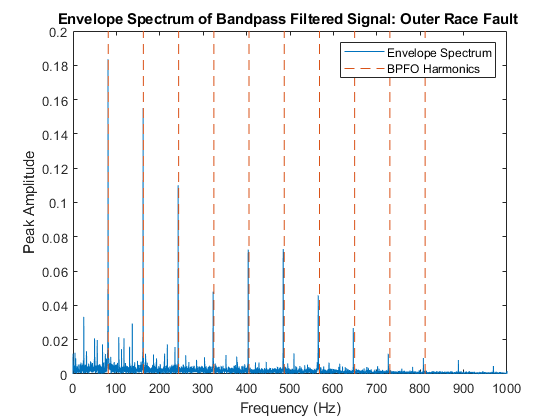
It is shown that by bandpass filtering the raw signal with the frequency band suggested by kurtogram and spectral kurtosis, the envelope spectrum analysis is able to reveal the fault signature at BPFO and its harmonics.

Batch Process

Now let's apply the algorithm to a batch of training data using a file ensemble datastore.

A limited portion of the dataset is available in the toolbox. Copy the dataset to the current folder and enable the write permission:

copyfile(...
    fullfile(matlabroot, 'toolbox', 'predmaint', 'predmaintdemos', ...
    'bearingFaultDiagnosis'), ...
    'RollingElementBearingFaultDiagnosis-Data-master')
fileattrib(fullfile('RollingElementBearingFaultDiagnosis-Data-master', 'train_data', '*.mat'), '+w')
fileattrib(fullfile('RollingElementBearingFaultDiagnosis-Data-master', 'test_data', '*.mat'), '+w')

For the full dataset, go to this link https://github.com/mathworks/RollingElementBearingFaultDiagnosis-Data to download the entire repository as a zip file and save it in the same directory as the live script. Unzip the file using this command:

if exist('RollingElementBearingFaultDiagnosis-Data-master.zip', 'file')
    unzip('RollingElementBearingFaultDiagnosis-Data-master.zip')
end

The results in this example are generated from the full dataset. The full dataset contains a training dataset with 14 mat files (2 normal, 4 inner race fault, 7 outer race fault) and a testing dataset with 6 mat files (1 normal, 2 inner race fault, 3 outer race fault).

By assigning function handles to ReadFcn and WriteToMemberFcn, the file ensemble datastore will be able to navigate into the files to retrieve data in the desired format. For example, the MFPT data has a structure bearing that stores the vibration signal gs, sampling rate sr, and so on. Instead of returning the bearing structure itself the readMFPTBearing function is written so that file ensemble datastore returns the vibration signal gs inside of the bearing data structure.

fileLocation = fullfile('.', 'RollingElementBearingFaultDiagnosis-Data-master', 'train_data');
fileExtension = '.mat';
ensembleTrain = fileEnsembleDatastore(fileLocation, fileExtension);
ensembleTrain.ReadFcn = @readMFPTBearing;
ensembleTrain.DataVariables = ["gs", "sr", "rate", "load", "BPFO", "BPFI", "FTF", "BSF"];
ensembleTrain.ConditionVariables = ["Label", "FileName"];
ensembleTrain.WriteToMemberFcn = @writeMFPTBearing;
ensembleTrain.SelectedVariables = ["gs", "sr", "rate", "load", "BPFO", "BPFI", "FTF", "BSF", "Label", "FileName"]

ensembleTrain = 
  fileEnsembleDatastore with properties:

                 ReadFcn: @readMFPTBearing
        WriteToMemberFcn: @writeMFPTBearing
           DataVariables: [8×1 string]
    IndependentVariables: [0×0 string]
      ConditionVariables: [2×1 string]
       SelectedVariables: [10×1 string]
                ReadSize: 1
              NumMembers: 14
          LastMemberRead: [0×0 string]
                   Files: [14×1 string]

ensembleTrainTable = tall(ensembleTrain)

Starting parallel pool (parpool) using the 'local' profile ...
connected to 6 workers.

ensembleTrainTable =

  M×10 tall table

           gs             sr      rate    load     BPFO      BPFI      FTF       BSF           Label                   FileName        
    _________________    _____    ____    ____    ______    ______    ______    _____    __________________    ________________________

    [146484×1 double]    48828     25       0     81.125    118.88    14.838    63.91    "Inner Race Fault"    "InnerRaceFault_vload_1"
    [146484×1 double]    48828     25      50     81.125    118.88    14.838    63.91    "Inner Race Fault"    "InnerRaceFault_vload_2"
    [146484×1 double]    48828     25     100     81.125    118.88    14.838    63.91    "Inner Race Fault"    "InnerRaceFault_vload_3"
    [146484×1 double]    48828     25     150     81.125    118.88    14.838    63.91    "Inner Race Fault"    "InnerRaceFault_vload_4"
    [146484×1 double]    48828     25     200     81.125    118.88    14.838    63.91    "Inner Race Fault"    "InnerRaceFault_vload_5"
    [585936×1 double]    97656     25     270     81.125    118.88    14.838    63.91    "Outer Race Fault"    "OuterRaceFault_1"      
    [585936×1 double]    97656     25     270     81.125    118.88    14.838    63.91    "Outer Race Fault"    "OuterRaceFault_2"      
    [146484×1 double]    48828     25      25     81.125    118.88    14.838    63.91    "Outer Race Fault"    "OuterRaceFault_vload_1"
            :              :       :       :        :         :         :         :              :                        :
            :              :       :       :        :         :         :         :              :                        :

From the last section of analysis, notice that the bandpass filtered envelope spectrum amplitudes at BPFO and BPFI are two condition indicators for bearing fault diagnosis. Therefore, the next step is to extract the two condition indicators from all the training data. To make the algorithm more robust, set a narrow band (bandwidth = $10 Δ f$ , where $Δ f$ is the frequency resolution of the power spectrum) around BPFO and BPFI, and then find the maximum amplitude inside this narrow band. The algorithm is contained in the bearingFeatureExtraction function listed below. Note that the envelope spectrum amplitudes around BPFI and BPFO are referred to as "BPFIAmplitude" and "BPFOAmplitude" in the rest of the example.

% To process the data in parallel, use the following code
% ppool = gcp;
% n = numpartitions(ensembleTrain, ppool);
% parfor ct = 1:n
%     subEnsembleTrain = partition(ensembleTrain, n, ct);
%     reset(subEnsembleTrain);
%     while hasdata(subEnsembleTrain)
%         bearingFeatureExtraction(subEnsembleTrain);
%     end
% end
ensembleTrain.DataVariables = [ensembleTrain.DataVariables; "BPFIAmplitude"; "BPFOAmplitude"];
reset(ensembleTrain)
while hasdata(ensembleTrain)
    bearingFeatureExtraction(ensembleTrain)
end

Once the new condition indicators are added into the file ensemble datastore, specify SelectedVariables to read the relevant data from the file ensemble datastore, and create a feature table containing the extracted condition indicators.

ensembleTrain.SelectedVariables = ["BPFIAmplitude", "BPFOAmplitude", "Label"];
featureTableTrain = tall(ensembleTrain);
featureTableTrain = gather(featureTableTrain);

Evaluating tall expression using the Parallel Pool 'local':
- Pass 1 of 1: 0% complete
Evaluation 0% complete

- Pass 1 of 1: Completed in 3 sec
Evaluation completed in 3 sec

featureTableTrain

featureTableTrain=14×3 table
    BPFIAmplitude    BPFOAmplitude          Label       
    _____________    _____________    __________________

        0.33918         0.082296      "Inner Race Fault"
        0.31488         0.026599      "Inner Race Fault"
        0.52356         0.036609      "Inner Race Fault"
        0.52899         0.028381      "Inner Race Fault"
        0.13515         0.012337      "Inner Race Fault"
       0.004024          0.03574      "Outer Race Fault"
      0.0044918           0.1835      "Outer Race Fault"
      0.0074993          0.30166      "Outer Race Fault"
       0.013662          0.12468      "Outer Race Fault"
      0.0070963          0.28215      "Outer Race Fault"
      0.0060772          0.35241      "Outer Race Fault"
       0.011244          0.17975      "Outer Race Fault"
      0.0036798        0.0050208      "Normal"          
        0.00359        0.0069449      "Normal"

Visualize the feature table that has been created.

figure
gscatter(featureTableTrain.BPFIAmplitude, featureTableTrain.BPFOAmplitude, featureTableTrain.Label, [], 'ox+')
xlabel('BPFI Amplitude')
ylabel('BPFO Amplitude')

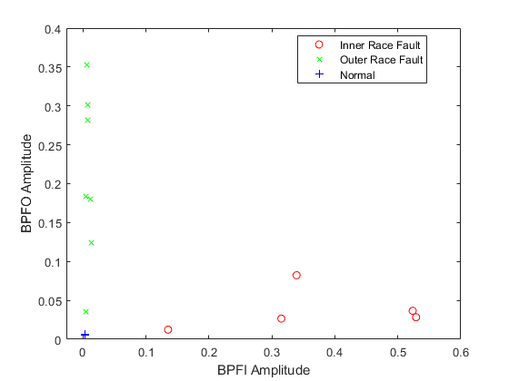
The relative values of BPFI Amplitude and BPFO Amplitude might be an effective indicator of different fault types. Here a new feature is created, which is the log ratio of the two existing features, and is visualized in a histogram grouped by different fault types.

featureTableTrain.IOLogRatio = log(featureTableTrain.BPFIAmplitude./featureTableTrain.BPFOAmplitude);
figure
hold on
histogram(featureTableTrain.IOLogRatio(featureTableTrain.Label=="Inner Race Fault"), 'BinWidth', 0.5)
histogram(featureTableTrain.IOLogRatio(featureTableTrain.Label=="Outer Race Fault"), 'BinWidth', 0.5)
histogram(featureTableTrain.IOLogRatio(featureTableTrain.Label=="Normal"), 'BinWidth', 0.5)
plot([-1.5 -1.5 NaN 0.5 0.5], [0 3 NaN 0 3], 'k--')
hold off
ylabel('Count')
xlabel('log(BPFIAmplitude/BPFOAmplitude)')
legend('Inner Race Fault', 'Outer Race Fault', 'Normal', 'Classification Boundary')

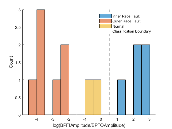
The histogram shows a clear separation among the three different bearing conditions. The log ratio between the BPFI and BPFO amplitudes is a valid feature to classify bearing faults. To simplify the example, a very simple classifier is derived: if $\log (\frac{BPFIAmp litude}{BPFOAmp litude}) \leq - 1.5$ , the bearing has an outer race fault; if $- 1.5 < \log (\frac{BPFIAmp litude}{BPFOAmp litude}) \leq 0.5$ , the bearing is normal; and if $\log (\frac{BPFIAmp litude}{BPFOAmp litude}) > 0.5$ , the bearing has an inner race fault.

Validation using Test Data Sets

Now, let's apply the workflow to a test data set and validate the classifier obtained in the last section. Here the test data contains 1 normal data set, 2 inner race fault data sets, and 3 outer race fault data sets.

fileLocation = fullfile('.', 'RollingElementBearingFaultDiagnosis-Data-master', 'test_data');
fileExtension = '.mat';
ensembleTest = fileEnsembleDatastore(fileLocation, fileExtension);
ensembleTest.ReadFcn = @readMFPTBearing;
ensembleTest.DataVariables = ["gs", "sr", "rate", "load", "BPFO", "BPFI", "FTF", "BSF"];
ensembleTest.ConditionVariables = ["Label", "FileName"];
ensembleTest.WriteToMemberFcn = @writeMFPTBearing;
ensembleTest.SelectedVariables = ["gs", "sr", "rate", "load", "BPFO", "BPFI", "FTF", "BSF", "Label", "FileName"]

ensembleTest = 
  fileEnsembleDatastore with properties:

                 ReadFcn: @readMFPTBearing
        WriteToMemberFcn: @writeMFPTBearing
           DataVariables: [8×1 string]
    IndependentVariables: [0×0 string]
      ConditionVariables: [2×1 string]
       SelectedVariables: [10×1 string]
                ReadSize: 1
              NumMembers: 6
          LastMemberRead: [0×0 string]
                   Files: [6×1 string]

ensembleTest.DataVariables = [ensembleTest.DataVariables; "BPFIAmplitude"; "BPFOAmplitude"];
reset(ensembleTest)
while hasdata(ensembleTest)
    bearingFeatureExtraction(ensembleTest)
end

ensembleTest.SelectedVariables = ["BPFIAmplitude", "BPFOAmplitude", "Label"];
featureTableTest = tall(ensembleTest);
featureTableTest = gather(featureTableTest);

Evaluating tall expression using the Parallel Pool 'local':
- Pass 1 of 1: Completed in 1 sec
Evaluation completed in 1 sec

featureTableTest.IOLogRatio = log(featureTableTest.BPFIAmplitude./featureTableTest.BPFOAmplitude);

figure
hold on
histogram(featureTableTrain.IOLogRatio(featureTableTrain.Label=="Inner Race Fault"), 'BinWidth', 0.5)
histogram(featureTableTrain.IOLogRatio(featureTableTrain.Label=="Outer Race Fault"), 'BinWidth', 0.5)
histogram(featureTableTrain.IOLogRatio(featureTableTrain.Label=="Normal"), 'BinWidth', 0.5)

histogram(featureTableTest.IOLogRatio(featureTableTest.Label=="Inner Race Fault"), 'BinWidth', 0.1)
histogram(featureTableTest.IOLogRatio(featureTableTest.Label=="Outer Race Fault"), 'BinWidth', 0.1)
histogram(featureTableTest.IOLogRatio(featureTableTest.Label=="Normal"), 'BinWidth', 0.1)
plot([-1.5 -1.5 NaN 0.5 0.5], [0 3 NaN 0 3], 'k--')
hold off
ylabel('Count')
xlabel('log(BPFIAmplitude/BPFOAmplitude)')
legend('Inner Race Fault - Train', 'Outer Race Fault - Train', 'Normal - Train', ...
    'Inner Race Fault - Test', 'Outer Race Fault - Test', 'Normal - Test', ...
    'Classification Boundary')

The log ratio of BPFI and BPFO amplitudes from test data sets shows consistent distribution with the log ratio from training data sets. The naive classifier obtained in the last section achieved perfect accuracy on the test data set.

It should be noted that single feature is usually not enough to get a classifier that generalizes well. More sophisticated classifiers could be obtained by dividing the data into multiple pieces (to create more data points), extract multiple diagnosis related features, select a subset of features by their importance ranks, and train various classifiers using the Classification Learner App in Statistics & Machine Learning Toolbox. For more details of this workflow, please refer to the example "Using Simulink to generate fault data".

Summary

This example shows how to use kurtogram, spectral kurtosis and envelope spectrum to identify different types of faults in rolling element bearings. The algorithm is then applied to a batch of data sets in disk, which helped show that the amplitudes of bandpass filtered envelope spectrum at BPFI and BPFO are two important condition indicators for bearing diagnostics.

References

[1] Randall, Robert B., and Jerome Antoni. "Rolling element bearing diagnostics—a tutorial." Mechanical Systems and Signal Processing. Vol. 25, Number 2, 2011, pp. 485–520.

[2] Antoni, Jérôme. "Fast computation of the kurtogram for the detection of transient faults." Mechanical Systems and Signal Processing. Vol. 21, Number 1, 2007, pp. 108–124.

[3] Antoni, Jérôme. "The spectral kurtosis: a useful tool for characterising non-stationary signals." Mechanical Systems and Signal Processing. Vol. 20, Number 2, 2006, pp. 282–307.

[4] Bechhoefer, Eric. "Condition Based Maintenance Fault Database for Testing Diagnostics and Prognostic Algorithms." 2013. https://www.mfpt.org/fault-data-sets/

Helper Functions

function bearingFeatureExtraction(ensemble)
% Extract condition indicators from bearing data
data = read(ensemble);
x = data.gs{1};
fs = data.sr;

% Critical Frequencies
BPFO = data.BPFO;
BPFI = data.BPFI;

level = 9;
[~, ~, ~, fc, ~, BW] = kurtogram(x, fs, level);

% Bandpass filtered Envelope Spectrum
[pEnvpBpf, fEnvBpf] = envspectrum(x, fs, 'FilterOrder', 200, 'Band', [max([fc-BW/2 0]) min([fc+BW/2 0.999*fs/2])]);
deltaf = fEnvBpf(2) - fEnvBpf(1);

BPFIAmplitude = max(pEnvpBpf((fEnvBpf > (BPFI-5*deltaf)) & (fEnvBpf < (BPFI+5*deltaf))));
BPFOAmplitude = max(pEnvpBpf((fEnvBpf > (BPFO-5*deltaf)) & (fEnvBpf < (BPFO+5*deltaf))));

writeToLastMemberRead(ensemble, table(BPFIAmplitude, BPFOAmplitude, 'VariableNames', {'BPFIAmplitude', 'BPFOAmplitude'}));
end