Data Ensembles for Condition Monitoring and Predictive Maintenance
Data analysis is the heart of any condition monitoring and predictive maintenance activity. Predictive Maintenance Toolbox™ provides tools called ensemble datastores for creating, labeling, and managing the often large, complex data sets needed for predictive maintenance algorithm design.
The data can come from measurements on systems using sensors such as accelerometers, pressure gauges, thermometers, altimeters, voltmeters, and tachometers. For instance, you might have access to measured data from:
Normal system operation
The system operating in a faulty condition
Lifetime record of system operation (run-to-failure data)
For algorithm design, you can also use simulated data generated by running a Simulink® model of your system under various operating and fault conditions.
Whether using measured data, generated data, or both, you frequently have many signals, ranging over a time span or multiple time spans. You might also have signals from many machines (for example, measurements from 100 separate engines all manufactured to the same specifications). And you might have data representing both healthy operation and fault conditions. In any case, designing algorithms for predictive maintenance requires organizing and analyzing large amounts of data while keeping track of the systems and conditions the data represents.
Ensemble datastores can help you work with such data, whether it is stored locally or in a remote location such as cloud storage using Amazon S3™ (Simple Storage Service), Windows Azure® Blob Storage, and Hadoop® Distributed File System (HDFS™).
Data Ensembles
The main unit for organizing and managing multifaceted data sets in Predictive Maintenance Toolbox is the data ensemble. An ensemble is a collection of data sets, created by measuring or simulating a system under varying conditions.
For example, consider a transmission gear box system in which you have an accelerometer to measure vibration and a tachometer to measure the engine shaft rotation. Suppose that you run the engine for five minutes and record the measured signals as a function of time. You also record the engine age, measured in miles driven. Those measurements yield the following data set.

Now suppose that you have a fleet of many identical engines, and you record data from all of them. Doing so yields a family of data sets.

This family of data sets is an ensemble, and each row in the ensemble is a member of the ensemble.
The members in an ensemble are related in that they contain the same data variables. For instance, in the illustrated ensemble, all members include the same four variables: an engine identifier, the vibration and tachometer signals, and the engine age. In that example, each member corresponds to a different machine. Your ensemble might also include that set of data variables recorded from the same machine at different times. For instance, the following illustration shows an ensemble that includes multiple data sets from the same engine recorded as the engine ages.

In practice, the data for each ensemble member is typically stored in a separate data file. Thus, for instance, you might have one file containing the data for engine 01 at 9,500 miles, another file containing the data for engine 01 at 21,250 miles, and so on.
Simulated Ensemble Data
In many cases, you have no real failure data from your system, or only limited data from the system in fault conditions. If you have a Simulink model that approximates the behavior of the actual system, you can generate a data ensemble by simulating the model repeatedly under various conditions and logging the simulation data. For instance, you can:
Vary parameter values that reflect the presence or absence of a fault. For example, use a very low resistance value to model a short circuit.
Injecting signal faults. Sensor drift and disturbances in the measured signal affect the measured data values. You can simulate such variation by adding an appropriate signal to the model. For example, you can add an offset to a sensor to represent drift, or model a disturbance by injecting a signal at some location in the model.
Vary system dynamics. The equations that govern the behavior of a component may change for normal and faulty operation. In this case, the different dynamics can be implemented as variants of the same component.
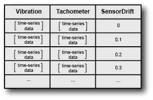
For example, suppose that you have a Simulink model that describes a gear-box system. The model contains a parameter that represents the drift in a vibration sensor. You simulate this model at different values of sensor drift, and configure the model to log the vibration and tachometer signals for each simulation. These simulations generate an ensemble that covers a range of operating conditions. Each ensemble member corresponds to one simulation, and records the same data variables under a particular set of conditions.
The generateSimulationEnsemble command helps you generate such data
sets from a model in which you can simulate fault conditions by varying some
aspect of the model.
Ensemble Variables
The variables in your ensemble serve different purposes, and accordingly can be grouped into several types:
Data variables — The main content of the ensemble members, including measured data and derived data that you use for analysis and development of predictive maintenance algorithms. For example, in the illustrated gear-box ensembles,
VibrationandTachometerare the data variables. Data variables can also include derived values, such as the mean value of a signal, or the frequency of the peak magnitude in a signal spectrum.Independent variables — The variables that identify or order the members in an ensemble, such as timestamps, number of operating hours, or machine identifiers. In the ensemble of measured gear-box data,
Ageis an independent variable.Condition variables — The variables that describe the fault condition or operating condition of the ensemble member. Condition variables can record the presence or absence of a fault state, or other operating conditions such as ambient temperature. In the ensemble of simulated gear-box data,
SensorDriftis a condition variable. Condition variables can also be derived values, such as a single scalar value that encodes multiple fault and operating conditions.
In practice, your data variables, independent variables, and condition variables are all distinct sets of variables.
Ensemble Data in Predictive Maintenance Toolbox
With Predictive Maintenance Toolbox, you manage and interact with ensemble data using ensemble
datastore objects. In MATLAB®, time-series data is often stored as a vector or a
timetable. Other data might be stored as scalar values (such
as engine age), logical values (such as whether a fault is present or not), strings
(such as an identifier), or tables. Your ensemble can contain any data type that is
useful to record for your application. In an ensemble, you typically store the data
for each member in a separate file. Ensemble datastore objects help you organize,
label, and process ensemble data. Which ensemble datastore object you use depends on
whether you are working with measured data on disk, or generating simulated data
from a Simulink model.
simulationEnsembleDatastoreobjects — Manage data generated from a Simulink model usinggenerateSimulationEnsemble.fileEnsembleDatastoreobjects — Manage any other ensemble data stored on disk, such as measured data.
The ensemble datastore objects contain information about the data stored on disk
and allow you to interact with the data. You do so using commands such as read, which extracts data from the ensemble into the MATLAB workspace, and writeToLastMemberRead, which writes data to the ensemble.
Last Member Read
When you work with an ensemble, the software keeps track of which ensemble
member it has most recently read. When you call read, the
software selects the next member to read and updates the
LastMemberRead property of the ensemble to reflect that
member. When you next call writeToLastMemberRead, the
software writes to that member.
For example, consider the ensemble of simulated gear-box data. When you
generate this ensemble using generateSimulationEnsemble,
the data from each simulation run is logged to a separate file on disk. You then
create a simulationEnsembleDatastore object that points to the
data in those files. You can set properties of the ensemble object to separate
the variables into groups such as independent variables or condition
variables.
Suppose that you now read some data from the ensemble object,
ensemble.
data = read(ensemble);
The first time you call read on an ensemble, the software
designates some member of the ensemble as the first member to read. The software
reads selected variables from that member into the MATLAB workspace, into a table called
data. (The selected variables are the variables you
specify in the SelectedVariables property of
ensemble.) The software updates the property
ensemble.LastMemberRead with the file name of that
member.

Until you call read again, the
last-member-read designation stays with the ensemble
member to which the software assigned it. Thus, for example, suppose that you
process data to compute some derived variable, such as the
frequency of the peak value in the vibration signal spectrum,
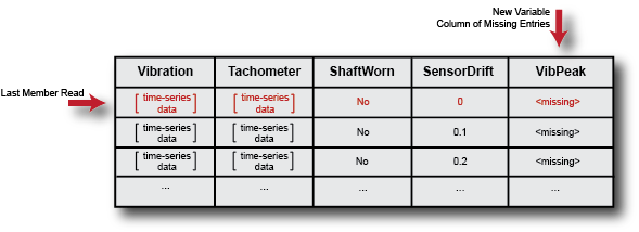
VibPeak. You can append the derived value to the ensemble
member to which it corresponds, which is still the last member read. To do so,
first expand the list of data variables in ensemble to
include the new variable.
ensemble.DataVariables = [ensemble.DataVariables; "VibPeak"]This operation is equivalent to adding a new column to the ensemble, as shown
in the next illustration. The new variable is initially populated in each
ensemble by a missing value. (See missing for more
information.)
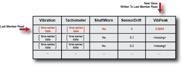
Now, use writeToLastMemberRead to fill in the value of
the new variable for the last member read.
newdata = table(VibPeak,'VariableNames',{'VibPeak'});
writeToLastMemberRead(ensemble,newdata);
In the ensemble, the new value is present, and the last-member-read designation remains on the same member.
The next time you call read on the ensemble, it
determines the next member to read, and returns the selected variables from that
member. The last-member-read designation advances to that member.

The hasdata command tells you whether all members of the
ensemble have been read. The reset command clears the
"read" designation from all members, such that the next call to
read operates on the first member of the ensemble. The
reset operation clears the LastMemberRead property of the
ensemble, but it does not change other ensemble properties such as
DataVariables or SelectedVariables. It
also does not change any data that you have written back to the ensemble. For an
example that shows more interactions with an ensemble of generated data, see
Generate and Use Simulated Data Ensemble.
Reading Measured Data
Although the previous discussion used a simulated ensemble as an example, the
last-member-read designation behaves the same way in ensembles of measured data
that you manage with fileEnsembleDatastore. However, when you
work with measured data, you have to provide information to tell the
read and writeToLastMemberRead
commands how your data is stored and organized on disk.
You do so by setting properties of the fileEnsembleDatastore
object to functions that you write. Set the ReadFcn
property to the handle of a function that describes how to read the data
variables from a data file. When you call read, it uses
this function to access the next ensemble file, and to read from it the
variables specified in the SelectedVariables property of
the ensemble datastore. Similarly, you use the
WriteToMemberFcn property of the
fileEnsembleDatastore object to provide a function that
describes how to write data to a member of the ensemble.
For examples that show these interactions with an ensemble of measured data on disk, see:
Ensembles and MATLAB Datastores
Ensembles in Predictive Maintenance Toolbox are a specialized kind of MATLAB datastore (see
Getting Started with Datastore). The read and writeToLastMemberRead commands have behavior that is specific to
ensemble datastores. Additionally, the following MATLAB datastore commands work with ensemble datastores the same as they
do with other MATLAB datastores.
hasdata— Determine whether an ensemble datastore has members that have not yet been read.reset— Restore an ensemble datastore to the state where no members have yet been read. In this state, there is no current member. Use this command to reread data you have already read from an ensemble.tall— Convert ensemble datastore to tall table. (See Tall Arrays for Out-of-Memory Data).progress— Determine what percentage of an ensemble datastore has been read.partition— Partition an ensemble datastore into multiple ensemble datastores for parallel computing. (For ensemble datastores, use thepartition(ds,n,index)syntax.)numpartitions— Determine number of datastore partitions.
Reading from Multiple Ensemble Members
By default, the read command returns data from one
ensemble member at a time. To process data from more than one ensemble member at
a time, set the ReadSize of the ensemble datastore object
to a value greater than 1. For instance, if you set
ReadSize to 3, then each call to
read returns a table with three rows, and designates
three ensemble members as last member read. For details, see the
fileEnsembleDatastore and
simulationEnsembleDatastore reference pages.
Convert Ensemble Data into Tall Tables
Some functions, such as many statistical analysis functions, can operate on data
in tall tables, which let you work with out-of-memory data that is backed by a
datastore. You can convert data from an ensemble datastore into a tall table for use
with such analysis commands using the tall command.
When working with large ensemble data, such as long time-series signals, you
typically process them member-by-member in the ensemble using
read and writeToLastMemberRead. You
process the data to compute some feature of the data that can serve as a useful
condition indicator for that ensemble member.
Typically, your condition indicator is a scalar value or some other value that
takes up less space in memory than the original unprocessed signal. Thus, once you
have written such values to your datastore, you can use tall
and gather to extract the condition indicators into memory for
further statistical processing, such as training a classifier.
For example, suppose that each member of your ensemble contains time-series
vibration data. For each member, you read the ensemble data and compute a condition
indicator that is a scalar value derived from a signal-analysis process. You write
the derived value back to the member. Suppose that the derived value is in an
ensemble variable called Indicator and a label containing
information about the ensemble member (such as a fault condition) is in a variable
called Label. To perform further analysis on the ensemble, you
can read the condition indicator and label into memory, without reading in the
larger vibration data. To do so, set the SelectedVariables
property of the ensemble to the variables you want to read. Then use
tall to create a tall table of the selected variables, and
gather to read the values into memory.
ensemble.SelectedVariables = ["Indicator","Label"];
featureTable = tall(ensemble);
featureTable = gather(featureTable);
The resulting variable featureTable is an ordinary table
residing in the MATLAB workspace. You can process it with any function that supports the
MATLAB table data type.
For examples that illustrate the use of tall and
gather to manipulate ensemble data for predictive
maintenance analysis, see:
Processing Ensemble Data
After organizing your data in an ensemble, the next step in predictive maintenance algorithm design is to preprocess the data to clean or transform it. Then you process the data further to extract condition indicators, which are data features that you can use to distinguish healthy from faulty operation. For more information, see:
See Also
fileEnsembleDatastore | simulationEnsembleDatastore | read | generateSimulationEnsemble