Using Simulink to Generate Fault Data
This example shows how to use a Simulink® model to generate fault and healthy data. The fault and healthy data is used to develop a condition monitoring algorithm. The example uses a transmission system and models a gear tooth fault, a sensor drift fault and shaft wear fault.
Transmission System Model
The transmission casing model uses Simscape™ Driveline™ blocks to model a simple transmission system. The transmission system consists of a torque drive, drive shaft, clutch, and high and low gears connected to an output shaft.
mdl = 'pdmTransmissionCasing';
open_system(mdl)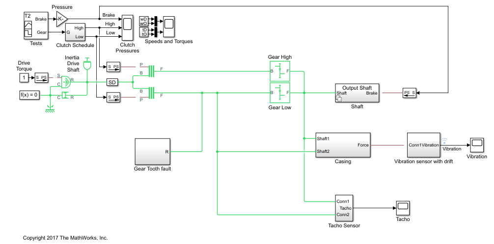
The transmission system includes a vibration sensor that is monitoring casing vibrations. The casing model translates the shaft angular displacement to a linear displacement on the casing. The casing is modeled as a mass spring damper system and the vibration (casing acceleration) is measured from the casing.
open_system([mdl '/Casing'])

Fault Modeling
The transmission system includes fault models for vibration sensor drift, gear tooth fault, and shaft wear. The sensor drift fault is easily modeled by introducing an offset in the sensor model. The offset is controlled by the model variable SDrift, note that SDrift=0 implies no sensor fault.
open_system([mdl '/Vibration sensor with drift'])
The shaft wear fault is modeled by a variant subsystem. In this case the subsystem variants change the shaft damping but the variant subsystem could be used to completely change the shaft model implementation. The selected variant is controlled by the model variable ShaftWear, note that ShaftWear=0 implies no shaft fault.
open_system([mdl '/Shaft'])
open_system([mdl,'/Shaft/Output Shaft'])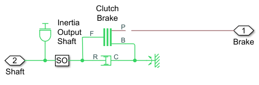
The gear tooth fault is modeled by injecting a disturbance torque at a fixed position in the rotation of the drive shaft. The shaft position is measured in radians and when the shaft position is within a small window around 0 a disturbance force is applied to the shaft. The magnitude of the disturbance is controlled by the model variable ToothFaultGain, note that ToothFaultGain=0 implies no gear tooth fault.

Simulating Fault and Healthy Data
The transmission model is configured with variables that control the presence and severity of the three different fault types, sensor drift, gear tooth, and shaft wear. By varying the model variables, SDrift, ToothFaultGain, and ShaftWear, you can create vibration data for the different fault types. Use an array of Simulink.SimulationInput objects to define a number of different simulation scenarios. For example, choose an array of values for each of the model variables and then use the ndgrid function to create a Simulink.SimulationInput for each combination of model variable values.
toothFaultArray = -2:2/10:0; % Tooth fault gain values
sensorDriftArray = -1:0.5:1; % Sensor drift offset values
shaftWearArray = [0 -1];       % Variants available for drive shaft conditions

% Create an n-dimensional array with combinations of all values
[toothFaultValues,sensorDriftValues,shaftWearValues] = ...
    ndgrid(toothFaultArray,sensorDriftArray,shaftWearArray);

for ct = numel(toothFaultValues):-1:1
    % Create a Simulink.SimulationInput for each combination of values
    siminput = Simulink.SimulationInput(mdl);

    % Modify model parameters
    siminput = setVariable(siminput,'ToothFaultGain',toothFaultValues(ct));
    siminput = setVariable(siminput,'SDrift',sensorDriftValues(ct));
    siminput = setVariable(siminput,'ShaftWear',shaftWearValues(ct));

    % Collect the simulation input in an array
    gridSimulationInput(ct) = siminput;
end
Similarly create combinations of random values for each model variable. Make sure to include the 0 value so that there are combinations where only subsets of the three fault types are represented.
rng('default'); % Reset random seed for reproducibility
toothFaultArray = [0 -rand(1,6)];    % Tooth fault gain values
sensorDriftArray = [0 randn(1,6)/8]; % Sensor drift offset values
shaftWearArray = [0 -1];               % Variants available for drive shaft conditions

%Create an n-dimensional array with combinations of all values
[toothFaultValues,sensorDriftValues,shaftWearValues] = ...
    ndgrid(toothFaultArray,sensorDriftArray,shaftWearArray);

for ct=numel(toothFaultValues):-1:1
    % Create a Simulink.SimulationInput for each combination of values
    siminput = Simulink.SimulationInput(mdl);

    % Modify model parameters
    siminput = setVariable(siminput,'ToothFaultGain',toothFaultValues(ct));
    siminput = setVariable(siminput,'SDrift',sensorDriftValues(ct));
    siminput = setVariable(siminput,'ShaftWear',shaftWearValues(ct));

    % Collect the simulation input in an array
    randomSimulationInput(ct) = siminput;
end
With the array of Simulink.SimulationInput objects defined use the generateSimulationEnsemble function to run the simulations. The generateSimulationEnsemble function configures the model to save logged data to file, use the timetable format for signal logging and store the Simulink.SimulationInput objects in the saved file. The generateSimulationEnsemble function returns a status flag indicating whether the simulation completed successfully.
The code above created 110 simulation inputs from the gridded variable values and 98 simulation inputs from the random variable values giving 208 total simulations. Running these 208 simulations in parallel can take as much as two hours or more on a standard desktop and generates around 10GB of data. An option to only run the first 10 simulations is provided for convenience.
% Run the simulations and create an ensemble to manage the simulation results
if ~exist(fullfile(pwd,'Data'),'dir')
    mkdir(fullfile(pwd,'Data')) % Create directory to store results
end
runAll = true;
if runAll
   [ok,e] = generateSimulationEnsemble([gridSimulationInput, randomSimulationInput], ...
        fullfile(pwd,'Data'),'UseParallel', true, 'ShowProgress', false);
else
    [ok,e] = generateSimulationEnsemble(gridSimulationInput(1:10), fullfile(pwd,'Data'), 'ShowProgress', false); %#ok<*UNRCH>
end
Starting parallel pool (parpool) using the 'Processes' profile ...
Preserving jobs with IDs: 1 because they contain crash dump files.
You can use 'delete(myCluster.Jobs)' to remove all jobs created with profile Processes. To create 'myCluster' use 'myCluster = parcluster('Processes')'.
Connected to parallel pool with 6 workers.
The generateSimulationEnsemble ran and logged the simulation results. Create a simulation ensemble to process and analyze the simulation results using the simulationEnsembleDatastore command.
ens = simulationEnsembleDatastore(fullfile(pwd,'Data'));Processing the Simulation Results
The simulationEnsembleDatastore command created an ensemble object that points to the simulation results. Use the ensemble object to prepare and analyze the data in each member of the ensemble. The ensemble object lists the data variables in the ensemble and by default all the variables are selected for reading.
ens
ens =
  simulationEnsembleDatastore with properties:

           DataVariables: [6×1 string]
    IndependentVariables: [0×0 string]
      ConditionVariables: [0×0 string]
       SelectedVariables: [6×1 string]
                ReadSize: 1
              NumMembers: 208
          LastMemberRead: [0×0 string]
                   Files: [208×1 string]
ens.SelectedVariables
ans = 6×1 string array
    "SimulationInput"
    "SimulationMetadata"
    "Tacho"
    "Vibration"
    "xFinal"
    "xout"
For analysis only read the Vibration and Tacho signals and the Simulink.SimulationInput. The Simulink.SimulationInput has the model variable values used for simulation and is used to create fault labels for the ensemble members. Use the ensemble read command to get the ensemble member data.
ens.SelectedVariables = ["Vibration" "Tacho" "SimulationInput"];
data = read(ens)
data=1×3 table
    40272×1 timetable    40272×1 timetable    1×1 SimulationInput
Extract the vibration signal from the returned data and plot it.
vibration = data.Vibration{1};
plot(vibration.Time,vibration.Data)
title('Vibration')
ylabel('Acceleration')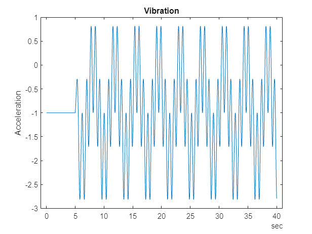
The first 10 seconds of the simulation contains data where the transmission system is starting up; for analysis discard this data.
idx = vibration.Time >= seconds(10);
vibration = vibration(idx,:);
vibration.Time = vibration.Time - vibration.Time(1);
The Tacho signal contains pulses for the rotations of the drive and load shafts but analysis, and specifically time synchronous averaging, requires the times of shaft rotations. The following code discards the first 10 seconds of the Tacho data and finds the shaft rotation times in tachoPulses.
tacho = data.Tacho{1};
idx = tacho.Time >= seconds(10);
tacho = tacho(idx,:);
plot(tacho.Time,tacho.Data)
title('Tacho pulses')
legend('Drive shaft','Load shaft') % Load shaft rotates more slowly than drive shaft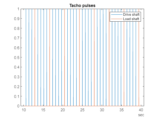
idx = diff(tacho.Data(:,2)) > 0.5;
tachoPulses = tacho.Time(find(idx)+1)-tacho.Time(1)
tachoPulses = 8×1 duration array
    "2.8543 sec"
    "6.6508 sec"
    "10.447 sec"
    "14.244 sec"
    "18.04 sec"
    "21.837 sec"
    "25.634 sec"
    "29.43 sec"
The Simulink.SimulationInput.Variables property contains the values of the fault parameters used for the simulation, these values allow us to create fault labels for each ensemble member.
vars = data.SimulationInput{1}.Variables;
idx = strcmp({vars.Name},'SDrift');
if any(idx)
    sF = abs(vars(idx).Value) > 0.01; % Small drift values are not faults
else
    sF = false;
end
idx = strcmp({vars.Name},'ShaftWear');
if any(idx)
    sV = vars(idx).Value < 0;
else
    sV = false;
end
if any(idx)
    idx = strcmp({vars.Name},'ToothFaultGain');
    sT = abs(vars(idx).Value) > 0.1; % Small tooth fault values are not faults
else
    sT = false
end
faultCode = sF + 2*sV + 4*sT; % A fault code to capture different fault conditions
The processed vibration and tacho signals and the fault labels are added to the ensemble to be used later.
sdata = table({vibration},{tachoPulses},sF,sV,sT,faultCode, ...
'VariableNames',{'Vibration','TachoPulses','SensorDrift','ShaftWear','ToothFault','FaultCode'}) sdata=1×6 table
30106×1 timetable 8×1 duration 1 0 0 1
ens.DataVariables = [ens.DataVariables; "TachoPulses"];The ensemble ConditionVariables property can be used to identify the variables in the ensemble that contain condition or fault label data. Set the property to contain the newly created fault labels.
ens.ConditionVariables = ["SensorDrift","ShaftWear","ToothFault","FaultCode"];
The code above was used to process one member of the ensemble. To process all the ensemble members the code above was converted to the function prepareData and using the ensemble hasdata command a loop is used to apply prepareData to all the ensemble members. The ensemble members can be processed in parallel by partitioning the ensemble and processing the ensemble partitions in parallel.
reset(ens)
runLocal = false;
if runLocal
    % Process each member in the ensemble
    while hasdata(ens)
        data = read(ens);
        addData = prepareData(data);
        writeToLastMemberRead(ens,addData)
    end
else
    % Split the ensemble into partitions and process each partition in parallel
    n = numpartitions(ens,gcp);
    parfor ct = 1:n
        subens = partition(ens,n,ct);
        while hasdata(subens)
            data = read(subens);
            addData = prepareData(data);
            writeToLastMemberRead(subens,addData)
        end
    end
end
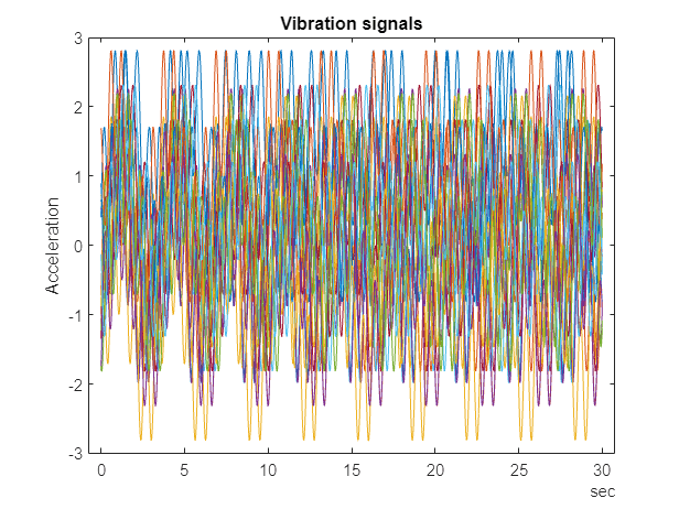
Plot the vibration signal of every 10th member of the ensemble using the hasdata and read commands to extract the vibration signal.
reset(ens)
ens.SelectedVariables = "Vibration";
figure,
ct = 1;
while hasdata(ens)
    data = read(ens);
    if mod(ct,10) == 0
        vibration = data.Vibration{1};
        plot(vibration.Time,vibration.Data)
        hold on
    end
    ct = ct + 1;
end
hold off
title('Vibration signals')
ylabel('Acceleration')
Analyzing the Simulation Data
Now that the data has been cleaned and pre-processed the data is ready for extracting features to determine the features to use to classify the different faults types. First configure the ensemble so that it only returns the processed data.
ens.SelectedVariables = ["Vibration","TachoPulses"];
For each member in the ensemble compute a number of time and spectrum based features. These include signal statistics such as signal mean, variance, peak to peak, non-linear signal characteristics such as approximate entropy and Lyapunov exponent, and spectral features such as the peak frequency of the time synchronous average of the vibration signal, and the power of the time synchronous average envelope signal. The analyzeData function contains a full list of the extracted features. By way of example consider computing the spectrum of the time synchronous averaged vibration signal.
reset(ens)
data = read(ens)
data=1×2 table
    30106×1 timetable    8×1 duration
vibration = data.Vibration{1};

% Interpolate the Vibration signal onto periodic time base suitable for fft analysis
np = 2^floor(log(height(vibration))/log(2));
dt = vibration.Time(end)/(np-1);
tv = 0:dt:vibration.Time(end);
y = retime(vibration,tv,'linear');

% Compute the time synchronous average of the vibration signal
tp = seconds(data.TachoPulses{1});
vibrationTSA = tsa(y,tp);
figure
plot(vibrationTSA.Time,vibrationTSA.tsa)
title('Vibration time synchronous average')
ylabel('Acceleration')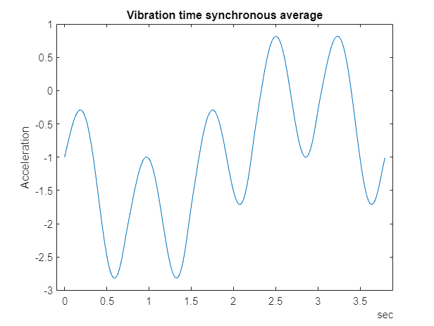
% Compute the spectrum of the time synchronous average
np = numel(vibrationTSA);
f = fft(vibrationTSA.tsa.*hamming(np))/np;
frTSA = f(1:floor(np/2)+1);            % TSA frequency response
wTSA = (0:np/2)/np*(2*pi/seconds(dt)); % TSA spectrum frequencies
mTSA = abs(frTSA);                     % TSA spectrum magnitudes
figure
semilogx(wTSA,20*log10(mTSA))
title('Vibration spectrum')
xlabel('rad/s')
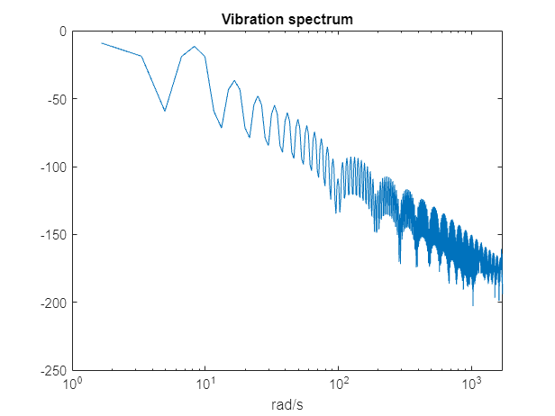
The frequency that corresponds to the peak magnitude could turn out to be a feature that is useful for classifying the different fault types. The code below computes the features mentioned above for all the ensemble members (running this analysis can take up to an hour on a standard desktop. Optional code to run the analysis in parallel using the ensemble partition command is provided.) The names of the features are added to the ensemble data variables property before calling writeToLastMemberRead to add the computed features to each ensemble member.
reset(ens)
ens.DataVariables = [ens.DataVariables; ...
    "SigMean";"SigMedian";"SigRMS";"SigVar";"SigPeak";"SigPeak2Peak";"SigSkewness"; ...
    "SigKurtosis";"SigCrestFactor";"SigMAD";"SigRangeCumSum";"SigCorrDimension";"SigApproxEntropy"; ...
    "SigLyapExponent";"PeakFreq";"HighFreqPower";"EnvPower";"PeakSpecKurtosis"];
if runLocal
    while hasdata(ens)
        data = read(ens);
        addData = analyzeData(data);
        writeToLastMemberRead(ens,addData);
    end
else
    % Split the ensemble into partitions and analyze each partition in parallel
    n = numpartitions(ens,gcp);
    parfor ct = 1:n
        subens = partition(ens,n,ct);
        while hasdata(subens)
            data = read(subens);
            addData = analyzeData(data);
            writeToLastMemberRead(subens,addData)
        end
    end
end
Selecting Features for Fault Classification
The features computed above are used to build a classifier to classify the different fault conditions. First configure the ensemble to read only the derived features and the fault labels.
featureVariables = analyzeData('GetFeatureNames');
ens.DataVariables = [ens.DataVariables; featureVariables];
ens.SelectedVariables = [featureVariables; ens.ConditionVariables];
reset(ens)
Gather the feature data for all the ensemble members into one table.
featureData = gather(tall(ens))
Evaluating tall expression using the Parallel Pool 'Processes':
- Pass 1 of 1: Completed in 14 sec
Evaluation completed in 14 sec
featureData=208×22 table
    -0.9488    -0.9722    1.3726    0.9839    0.8157    3.6314    -0.0415    2.2666    2.0514    0.8081    2.8562e+04    1.1427    0.0316     79.5312    0    6.7528e-06    3.2349e-07    162.1284    1    0    0    1
    -0.9754    -0.9896    1.3937    0.9911    0.8157    3.6314    -0.0238    2.2598    2.0203    0.8102    2.9418e+04    1.1362    0.0378     70.3389    0    5.0788e-08    9.1568e-08    226.1212    1    0    0    1
     1.0502     1.0267    1.4449    0.9849    2.8157    3.6314    -0.0416    2.2658    1.9487    0.8085    3.1710e+04    1.1479    0.0316    125.1842    0    6.7416e-06    3.1343e-07    162.1259    1    1    0    3
     1.0227     1.0045    1.4288    0.9955    2.8157    3.6314    -0.0164    2.2483    1.9707    0.8132    3.0984e+04    1.1472    0.0321    112.5155    0    4.9939e-06    2.6719e-07    162.1277    1    1    0    3
     1.0123     1.0024    1.4202    0.9923    2.8157    3.6314    -0.0147    2.2542    1.9826    0.8116    3.0661e+04    1.1470    0.0329    109.0188    0    3.6182e-06    2.1964e-07    230.3912    1    1    0    3
     1.0275     1.0102    1.4338    1.0001    2.8157    3.6314    -0.0266    2.2439    1.9638    0.8159    3.1102e+04    1.0975    0.0334     64.4981    0    2.5493e-06    1.9224e-07    230.3907    1    1    0    3
     1.0464     1.0275    1.4477    1.0011    2.8157    3.6314    -0.0428    2.2455    1.9449    0.8159    3.1665e+04    1.1417    0.0342     98.7589    0    1.7313e-06    1.6263e-07    230.3870    1    1    0    3
     1.0459     1.0257    1.4402    0.9805    2.8157    3.6314    -0.0354    2.2757    1.9550    0.8058    3.1554e+04    1.1345    0.0353     44.3035    0    1.1115e-06    1.2807e-07    230.3927    1    1    0    3
     1.0263     1.0068    1.4271    0.9834    2.8157    3.6314    -0.0165    2.2726    1.9730    0.8062    3.0951e+04    1.1515    0.0359    125.2802    0    6.5947e-07    1.2080e-07    162.1264    1    1    0    3
     1.0103     1.0014    1.4183    0.9909    2.8157    3.6314    -0.0117    2.2614    1.9853    0.8099    3.0465e+04    1.0619    0.0365     17.0927    0    5.2297e-07    1.0704e-07    230.3865    1    1    0    3
     1.0129     1.0023    1.4190    0.9876    2.8157    3.6314    -0.0110    2.2660    1.9843    0.8087    3.0523e+04    1.1371    0.0372     84.5701    0    2.1605e-07    8.5562e-08    230.3923    1    1    0    3
     1.0251     1.0104    1.4291    0.9917    2.8157    3.6314    -0.0236    2.2588    1.9702    0.8105    3.0896e+04    1.1261    0.0378     98.4616    0    5.0275e-08    9.0495e-08    230.3920    1    1    0    3
    -0.9730    -0.9924    1.3928    0.9933    0.8157    3.6314    -0.0126    2.2589    2.0216    0.8110    2.9351e+04    1.1277    0.0385     42.8867    0    1.1383e-11    8.3005e-08    230.3910    1    0    1    5
     1.0277     1.0084    1.4315    0.9931    2.8157    3.6314    -0.0135    2.2598    1.9669    0.8108    3.0963e+04    1.1486    0.0385     99.4258    0    1.1346e-11    8.3530e-08    226.1215    1    1    1    7
      ⋮
Consider the sensor drift fault. Use the fscnca command with all the features computed above as predictors and the sensor drift fault label (a true false value) as the response. The fscnca command returns weights for each feature and features with higher weights have higher importance in predicting the response. For the sensor drift fault the weights indicate that two features are significant predictors (the signal cumulative sum range and the peak frequency of the spectral kurtosis) and the remaining features have little impact.
idxResponse = strcmp(featureData.Properties.VariableNames,'SensorDrift');
idxLastFeature = find(idxResponse)-1; % Index of last feature to use as a potential predictor
featureAnalysis = fscnca(featureData{:,1:idxLastFeature},featureData.SensorDrift);
featureAnalysis.FeatureWeights
ans = 18×1

    0.0000
    0.0000
    0.0000
    0.0000
    0.0000
    0.0000
    0.0000
    0.0000
    0.0000
    0.0000
      ⋮
idxSelectedFeature = featureAnalysis.FeatureWeights > 0.1;
classifySD = [featureData(:,idxSelectedFeature), featureData(:,idxResponse)]
classifySD=208×3 table
    2.8562e+04    162.1284    1
    2.9418e+04    226.1212    1
    3.1710e+04    162.1259    1
    3.0984e+04    162.1277    1
    3.0661e+04    230.3912    1
    3.1102e+04    230.3907    1
    3.1665e+04    230.3870    1
    3.1554e+04    230.3927    1
    3.0951e+04    162.1264    1
    3.0465e+04    230.3865    1
    3.0523e+04    230.3923    1
    3.0896e+04    230.3920    1
    2.9351e+04    230.3910    1
    3.0963e+04    226.1215    1
      ⋮
A grouped histogram of the cumulative sum range gives us insight into why this feature is a significant predictor for the sensor drift fault.
figure
histogram(classifySD.SigRangeCumSum(classifySD.SensorDrift),'BinWidth',5e3)
xlabel('Signal cumulative sum range')
ylabel('Count')
hold on
histogram(classifySD.SigRangeCumSum(~classifySD.SensorDrift),'BinWidth',5e3)
hold off
legend('Sensor drift fault','No sensor drift fault')
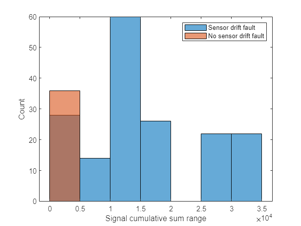
The histogram plot shows that the signal cumulative sum range is a good featured for detecting sensor drift faults though an additional feature is probably needed as there may be false positives when the signal cumulative sum range is below 0.5 if just the signal cumulative sum range is used to classify sensor drift.
Consider the shaft wear fault. In this case the fscnca function indicates that there are 3 features that are significant predictors for the fault (the signal Lyapunov exponent, peak frequency, and the peak frequency in the spectral kurtosis), choose these to classify the shaft wear fault.
idxResponse = strcmp(featureData.Properties.VariableNames,'ShaftWear');
featureAnalysis = fscnca(featureData{:,1:idxLastFeature},featureData.ShaftWear);
featureAnalysis.FeatureWeights
ans = 18×1
0.0000
0.0000
0.0000
0.0000
0.0000
0.0000
0.0000
0.0000
0.0000
0.0000
⋮
idxSelectedFeature = featureAnalysis.FeatureWeights > 0.1;
classifySW = [featureData(:,idxSelectedFeature), featureData(:,idxResponse)]
classifySW=208×4 table
     79.5312    0    162.1284    0
     70.3389    0    226.1212    0
    125.1842    0    162.1259    1
    112.5155    0    162.1277    1
    109.0188    0    230.3912    1
     64.4981    0    230.3907    1
     98.7589    0    230.3870    1
     44.3035    0    230.3927    1
    125.2802    0    162.1264    1
     17.0927    0    230.3865    1
     84.5701    0    230.3923    1
     98.4616    0    230.3920    1
     42.8867    0    230.3910    0
     99.4258    0    226.1215    1
      ⋮
The grouped histogram for the signal Lyapunov exponent shows why that feature alone is not a good predictor.
figure
histogram(classifySW.SigLyapExponent(classifySW.ShaftWear))
xlabel('Signal lyapunov exponent')
ylabel('Count')
hold on
histogram(classifySW.SigLyapExponent(~classifySW.ShaftWear))
hold off
legend('Shaft wear fault','No shaft wear fault')
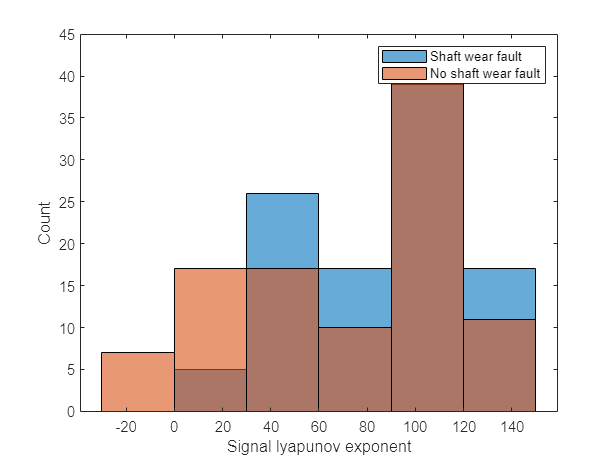
The shaft wear feature selection indicates multiple features are needed to classify the shaft wear fault, the grouped histogram confirms this as the most significant feature (in this case the Lyapunov exponent) has a similar distribution for both faulty and fault free scenarios indicating that more features are needed to correctly classify this fault.
Finally consider the tooth fault, the fscnca function indicates that there are 3 features primary that are significant predictors for the fault (the signal cumulative sum range, the signal Lyapunov exponent and the peak frequency in the spectral kurtosis). Choosing those 3 features to classify the tooth fault results in a classifier that has poor performance. Instead, use the 6 most important features.
idxResponse = strcmp(featureData.Properties.VariableNames,'ToothFault');
featureAnalysis = fscnca(featureData{:,1:idxLastFeature},featureData.ToothFault);
[~,idxSelectedFeature] = sort(featureAnalysis.FeatureWeights);
classifyTF = [featureData(:,idxSelectedFeature(end-5:end)), featureData(:,idxResponse)]classifyTF=208×7 table
0.8157 0 1.1427 79.5312 162.1284 2.8562e+04 0
0.8157 0 1.1362 70.3389 226.1212 2.9418e+04 0
2.8157 0 1.1479 125.1842 162.1259 3.1710e+04 0
2.8157 0 1.1472 112.5155 162.1277 3.0984e+04 0
2.8157 0 1.1470 109.0188 230.3912 3.0661e+04 0
2.8157 0 1.0975 64.4981 230.3907 3.1102e+04 0
2.8157 0 1.1417 98.7589 230.3870 3.1665e+04 0
2.8157 0 1.1345 44.3035 230.3927 3.1554e+04 0
2.8157 0 1.1515 125.2802 162.1264 3.0951e+04 0
2.8157 0 1.0619 17.0927 230.3865 3.0465e+04 0
2.8157 0 1.1371 84.5701 230.3923 3.0523e+04 0
2.8157 0 1.1261 98.4616 230.3920 3.0896e+04 0
0.8157 0 1.1277 42.8867 230.3910 2.9351e+04 1
2.8157 0 1.1486 99.4258 226.1215 3.0963e+04 1
⋮
figure
histogram(classifyTF.SigRangeCumSum(classifyTF.ToothFault))
xlabel('Signal cumulative sum range')
ylabel('Count')
hold on
histogram(classifyTF.SigRangeCumSum(~classifyTF.ToothFault))
hold off
legend('Gear tooth fault','No gear tooth fault')
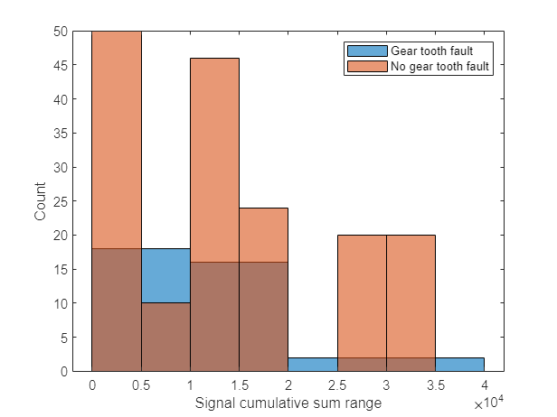
Using the above results a polynomial svm to classify gear tooth faults. Split the feature table into members that are used for training and members for testing and validation. Use the training members to create a svm classifier using the fitcsvm command.
rng('default') % For reproducibility
cvp = cvpartition(size(classifyTF,1),'KFold',5); % Randomly partition the data for training and validation
classifierTF = fitcsvm(...
    classifyTF(cvp.training(1),1:end-1), ...
    classifyTF(cvp.training(1),end), ...
    'KernelFunction','polynomial', ...
    'PolynomialOrder',2, ...
    'KernelScale','auto', ...
    'BoxConstraint',1, ...
    'Standardize',true, ...
    'ClassNames',[false; true]);
Use the classifier to classify the test points using the predict command and check the performance of the predictions using a confusion matrix.
% Use the classifier on the test validation data to evaluate performance
actualValue = classifyTF{cvp.test(1),end};
predictedValue = predict(classifierTF, classifyTF(cvp.test(1),1:end-1));

% Check performance by computing and plotting the confusion matrix
confdata = confusionmat(actualValue,predictedValue);
h = heatmap(confdata, ...
    'YLabel', 'Actual gear tooth fault', ...
    'YDisplayLabels', {'False','True'}, ...
    'XLabel', 'Predicted gear tooth fault', ...
    'XDisplayLabels', {'False','True'}, ...
    'ColorbarVisible','off');

The confusion matrix indicates that the classifier correctly classifies all non-fault conditions but incorrectly classifies one expected fault condition as not being a fault. Increasing the number of features used in the classifier can help improve the performance further.
Summary
This example walked through the workflow for generating fault data from Simulink, using a simulation ensemble to clean up the simulation data and extract features. The extracted features were then used to build classifiers for the different fault types.