Perform Prognostic Feature Ranking for a Degrading System Using Diagnostic Feature Designer

This example shows how to process and extract features from segmented data that contains evidence of a worsening shaft fault, and how to perform prognostic ranking to determine which features are best for determining remaining useful life (RUL). RUL feature development is based on run-to-failure data rather than conditionally grouped data.

The example assumes that you are already familiar with basic operations with the app. For a tutorial on using the app, see Design Condition Indicators for Predictive Maintenance Algorithms.

Model Description

The following figure illustrates a drivetrain with six gears. The motor for the drivetrain is fitted with a vibration sensor. The drivetrain has no tachometer. The motor drives a constant rotation speed of 1800 rpm with no variation. In this drivetrain:

Gear 1 on the motor shaft meshes with gear 2 with a gear ratio of 17:1.
The final gear ratio, or the ratio between gears 1 and 2 and gears 3 and 4, is 51:1.
Gear 5, also on the motor shaft, meshes with gear 6 with a gear ratio of 10:1.

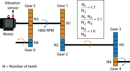
Ten simulated machines use this drivetrain. All of the machines have a fault developing on the shaft of gear 6. This fault becomes worse every day. The rate of the fault progression is fixed for each machine, but varies over the set of machines.

Data has been recorded during one 0.21 s period each day for 15 days. For each machine, these daily segments are stored in adjacent positions within a single variable. The timestamps reflect the data recording time and increase continuously. For instance, if the timestamp on the final sample of day 1 is t_f and the sample time is T_s, then the timestamp on the first sample of day 2 is t_f + T_s.

Import and View the Data

To start, load the data into your MATLAB^® workspace and open Diagnostic Feature Designer.

load(fullfile(matlabroot, 'toolbox', 'predmaint', 'predmaintdemos', ...
  'motorDrivetrainDiagnosis', 'machineDataRUL3'), 'motor_rul3')
diagnosticFeatureDesigner

Import the data. To do so, in the Feature Designer tab, click New Session. Then, in the Select more variables area of the New Session window, select motor_rul3 as your source variable.

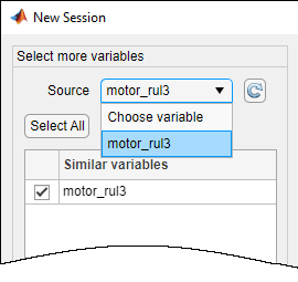
Complete the import process by accepting the default configuration and variables. The ensemble consists of one data variable Signal/vib, which contains the vibration signal. There are no condition variables.

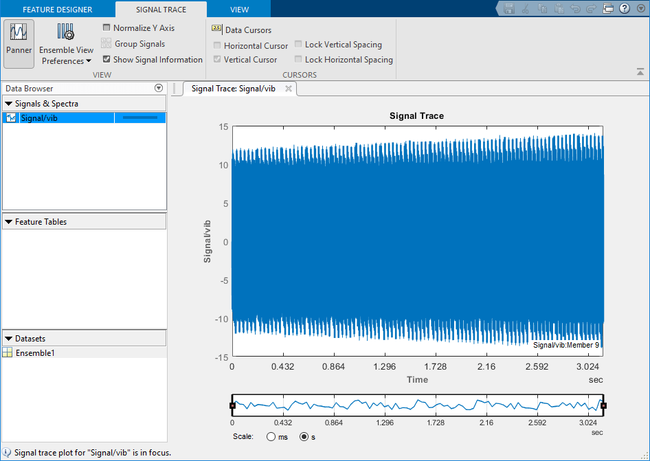
View the vibration signal. To do so, in the Data Browser, select the signal and plot it using Signal Trace. The amplitude of the signal increases continuously as the defect progresses.

Separate Daily Segments by Frame

When developing features for RUL use, you are interested in tracking the progression of degradation rather than in isolating specific faults. The time history of a useful RUL feature provides visibility into the degradation rate, and ultimately enables the projection of time to failure.

Frame-based processing allows you to track the progression of degradation segment by segment. Small or abrupt changes are captured in the segment that they occur. Segment-based features convey a more precise record of the degradation than features extracted from the full signal can provide. For RUL prediction, the progression rate of the degradation is as important as the magnitude of the defect at a given time.

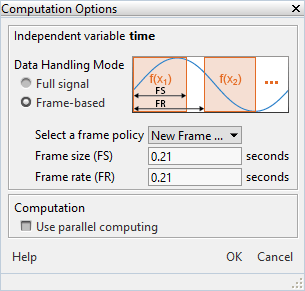
The data set for each machine in supports segmented processing by providing a segment of data for each day. Specify frame-based processing so that each of these segments is processed separately. Since the data has been collected in 0.21 s segments, separate the data for processing into 0.21 s frames.

Click Computation Options. In the dialog box, set Data Handling Mode to Frame-based. The data segments are contiguous, so set both the frame size and frame rate to 0.21 seconds.

Perform Time-Synchronous Averaging

Time-synchronous averaging (TSA) averages a signal over one rotation, substantially reducing noise that is not coherent with the rotation. TSA-filtered signals provide the basis for much rotational-machinery analysis, including feature generation.

In this example, the rotation speed is fixed to the same 1800 rpm value for each machine.

To compute the TSA signal, select Filtering & Averaging > Time-Synchronous Signal Averaging. In the dialog box:

Confirm the selection in Signal.
In Tacho Information, select Constant rotation speed (RPM) and set the value to 1800.
Accept all other settings.

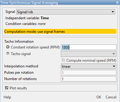
The app computes the TSA signal for each segment separately, and by default plots the first segment.

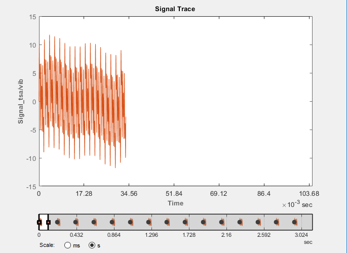
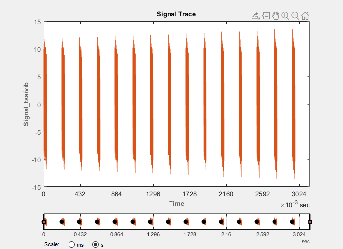
Use the panner to expand the plot to all segments. The plot shows a slightly increasing amplitude.

Extract Rotating Machinery Features

Use the TSA signal to compute time-domain rotating machinery features.

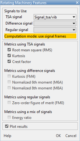
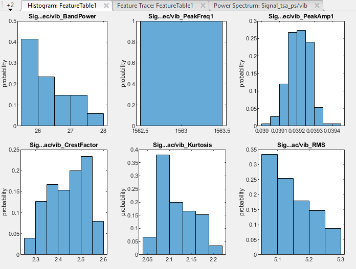
Since you have no condition variables, the resulting histograms display only the distribution of the feature values across the segments.

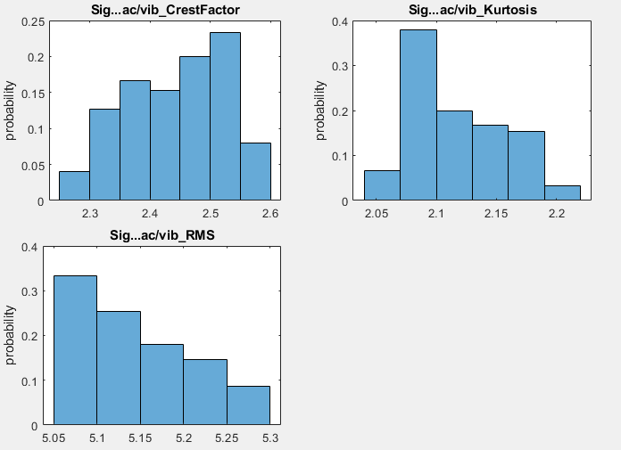
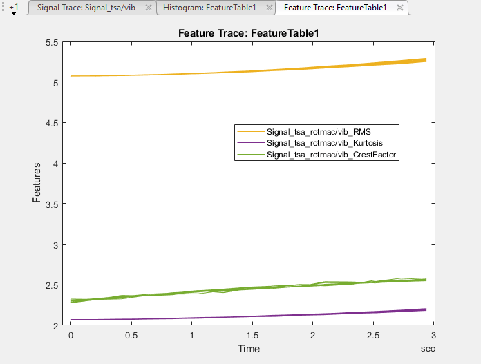
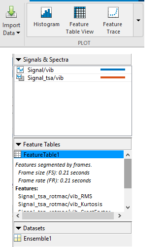
You can also look at the feature trace plots to see how the features change over time. To do so, in Feature Tables, select FeatureTable1. In the plot gallery, select Feature Trace.

In the feature trace plot, all three features show an upward slope corresponding to the continuing degradation. The values of the features relative to one another have no meaning, as the features represent different metrics that are not normalized.

Extract Spectral Features

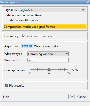
Spectral features generally work well when a defect results in a periodic oscillation. Extract spectral features from your TSA signal. Start by computing a power spectrum. To do so, select Spectral Estimation > Power Spectrum. Select the TSA signal and change Algorithm to Welch's method.

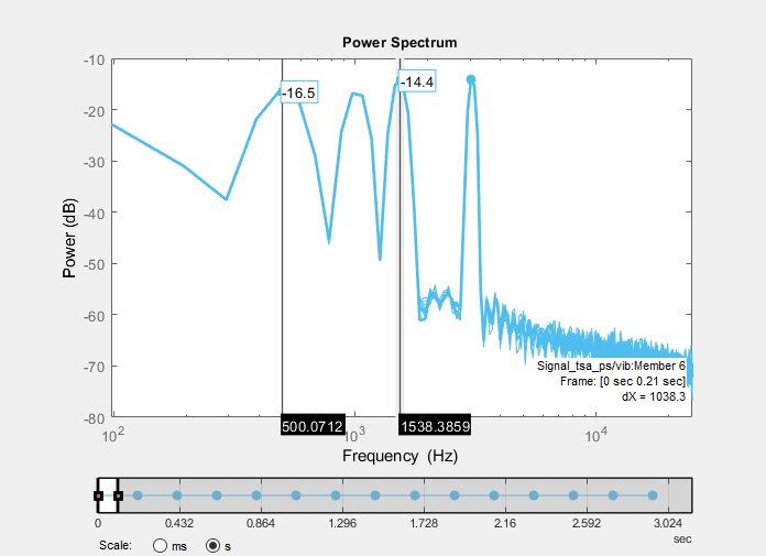
The spectrum for the first segment includes distinct peaks at around 500 Hz and 1540 Hz. The rotation speed is 1800 rpm or 30 Hz. The ratios between these peak frequencies are roughly 17 and 51, consistent with the gear ratios. The intervening peaks are additional harmonics of those frequencies.

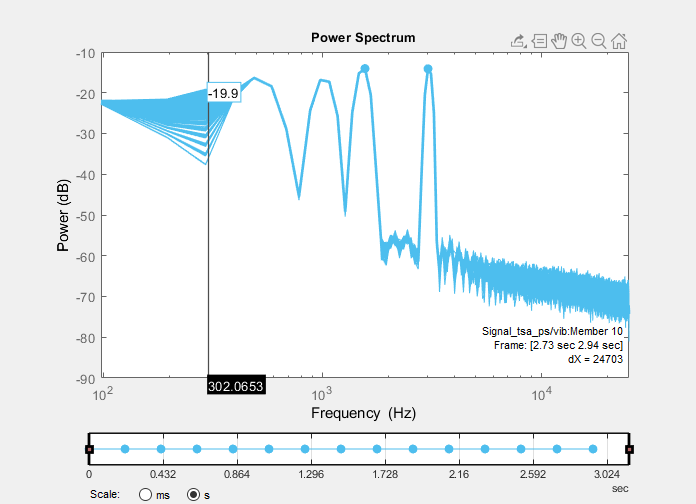
In the order and frequency domains, the segment spectra are superposed. The panner allows you to select multiple segments just as it does in the time domain. Set the panner to cover all the segments. As you expand the number of segments, the power increases at 300 Hz. This frequency corresponds to an order of 10 with respect to the 30 Hz rotation rate, and represents the increasing defect.

Extract spectral features. To do so, click Spectral Features and confirm that Spectrum is set to your power spectrum. Using the slider, limit the range to about 4000 Hz to bound the region to the peaks. The power spectrum plot automatically changes from a log to a linear scale and zooms in to the range you select.

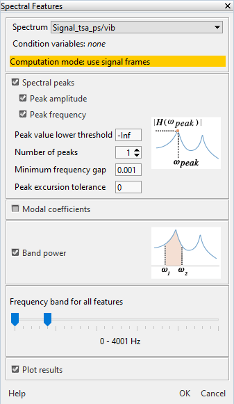
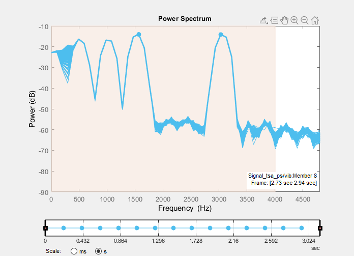
The resulting histogram plot now includes the spectral features.

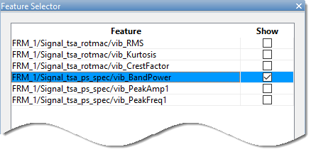
Plot the band-power feature trace to see how it compares with the all-segment power spectrum. Use Select Features to clear the other feature traces.

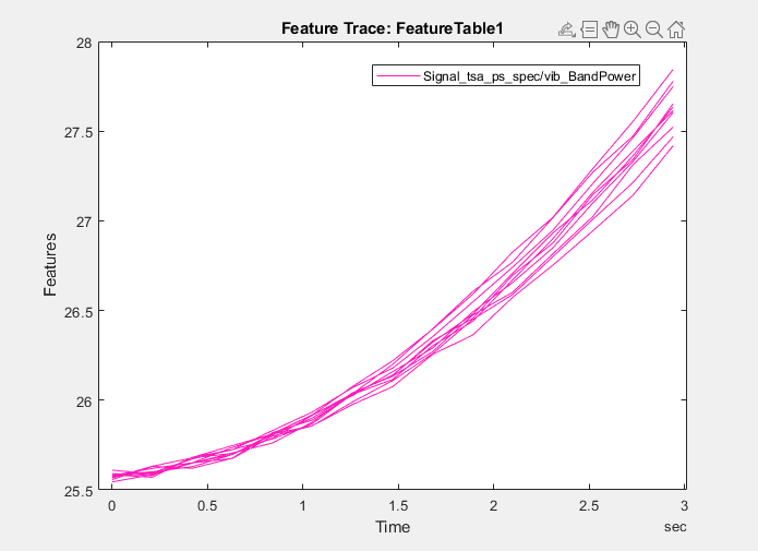
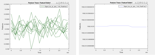
The band-power feature captures the progression of the defects in each machine. The traces of the other two spectral features do not track defect progression.

Rank Features with Prognostic Ranking Methods

Rank the features to see which ones perform best for predicting RUL. The app provides three prognostic ranking methods:

Monotonicity characterizes the trend of a feature as the system evolves toward failure. As a system gets progressively closer to failure, a suitable condition indicator has a monotonic positive or negative trend. For more information, see monotonicity.
Trendability provides a measure of similarity between the trajectories of a feature measured in multiple run-to-failure experiments. The trendability of a candidate condition indicator is defined as the smallest absolute correlation between measurements. For more information, see trendability.
Prognosability is a measure of the variability of a feature at failure relative to the range between its initial and final values. A more prognosable feature has less variation at failure relative to the range between its initial and final values. For more information, see prognosability.

Click Rank Features and select FeatureTable1. Because you have no condition variables, the app defaults to the prognostic ranking technique Monotonicity.

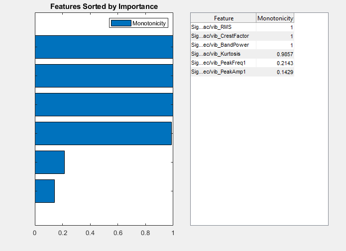
Four of the features score at or close to the maximum. Two features, PeakAmp1 and PeakFreq1, have considerably lower scores.

Add rankings for the other two prognostic methods. Click Prognostic Ranking and select Trendability. Click Apply and then Close Trendability.

Repeat the previous step for Prognosability. The ranking plot now contains the results of all three ranking methods.

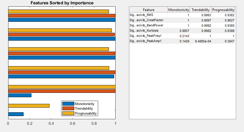
The ranking results are consistent with the feature traces plotted in Extract Spectral Features.

The features that track the worsening fault have high scores for Monotonicity. These features also have high scores for the other two methods.
PeakFreq1, which has the second lowest ranking Monotonicity score, has high scores for both Trendability and Prognosability. These high scores result from the close agreement among feature trajectories and low variability at the end of the simulation, where the fault is greatest.
PeakAmp1 has low scores for all rankings, reflecting both the insensitivity of this feature to defect progression and the variation in the machine values for this feature.

Since you have four features which scored well in all categories, choose these features as the feature set to move ahead with in an RUL algorithm.