monotonicity

In this example, consider the lifetime data of 10 identical machines with the following 6 potential prognostic parameters—constant, linear, quadratic, cubic, logarithmic, and periodic. The data set machineDataCellArray.mat contains C, which is a 1x10 cell array of matrices where each element of the cell array is a matrix that contains the lifetime data of a machine. For each matrix in the cell array, the first column contains the time while the other columns contain the data variables.

Load the lifetime data and visualize it against time.

load('machineDataCellArray.mat','C')
display(C)

C=1×10 cell array
    {219x7 double}    {189x7 double}    {202x7 double}    {199x7 double}    {229x7 double}    {184x7 double}    {224x7 double}    {208x7 double}    {181x7 double}    {197x7 double}

for k = 1:length(C)
    plot(C{k}(:,1), C{k}(:,2:end));
    hold on;
end

Observe the 6 different condition indicators—constant, linear, quadratic, cubic, logarithmic, and periodic—for all 10 machines on the plot.

Visualize the monotonicity of the potential prognostic features.

monotonicity(C)

From the histogram plot, observe that the features Var2, Var4 and Var5 rank better than the others. Hence, these features are more appropriate for remaining useful life predictions since they are the best indicators of machine health.

In this example, consider the lifetime data of 10 identical machines with the following 6 potential prognostic parameters—constant, linear, quadratic, cubic, logarithmic, and periodic. The data set machineDataTable.mat contains T, which is a 1x10 cell array of tables where each element of the cell array contains a table of lifetime data for a machine.

Load and display the data.

load('machineDataTable.mat','T');
display(T)

T=1×10 cell array
    {219x7 table}    {189x7 table}    {202x7 table}    {199x7 table}    {229x7 table}    {184x7 table}    {224x7 table}    {208x7 table}    {181x7 table}    {197x7 table}

head(T{1},2)

    Time    Constant    Linear    Quadratic    Cubic     Logarithmic    Periodic
    ____    ________    ______    _________    ______    ___________    ________

       0     3.2029     11.203     7.7029      3.8829      2.2517        0.2029 
    0.05     2.8135     10.763     7.2637      3.6006      1.8579       0.12251 

Note that every table in the cell array contains the lifetime variable 'Time' and the data variables 'Constant', 'Linear', 'Quadratic', 'Cubic', 'Logarithmic', and 'Periodic'.

Compute monotonicity using Spearman's rank correlation method with Time as the lifetime variable.

Y = monotonicity(T,'Time','Method','rank')

Y=1×6 table
    Constant    Linear    Quadratic     Cubic     Logarithmic    Periodic
    ________    ______    _________    _______    ___________    ________

    0.069487      1        0.17766     0.97993      0.99957      0.059208

From the resulting table of monotonicity values, observe that the linear, cubic, and logarithmic features have values closer to 1. Hence, these three features are more appropriate for predicting remaining useful life since they are the best indicators of machine health.

Consider the lifetime data of 4 machines. Each machine has 4 fault codes for the potential condition indicators—voltage, current, and power. monotonicityEnsemble.zip is a collection of 4 files where every file contains a timetable of lifetime data for each machine—tbl1.mat, tbl2.mat, tbl3.mat, and tbl4.mat. You can also use files containing data for multiple machines. For each timetable, the organization of the data is as follows:

When you perform calculations on tall arrays, MATLAB® uses either a parallel pool (default if you have Parallel Computing Toolbox™) or the local MATLAB session. To run the example using the local MATLAB session, change the global execution environment by using the mapreducer function.

mapreducer(0)

Extract the compressed files, read the data in the timetables, and create a fileEnsembleDatastore object using the timetable data. For more information on creating a file ensemble datastore, see fileEnsembleDatastore.

unzip monotonicityEnsemble.zip;
ens = fileEnsembleDatastore(pwd,'.mat');
ens.DataVariables = {'Voltage','Current','Power','FaultCode','Machine'};
ens.ReadFcn = @readtable_data;
ens.SelectedVariables = {'Voltage','Current','Power','FaultCode','Machine'};

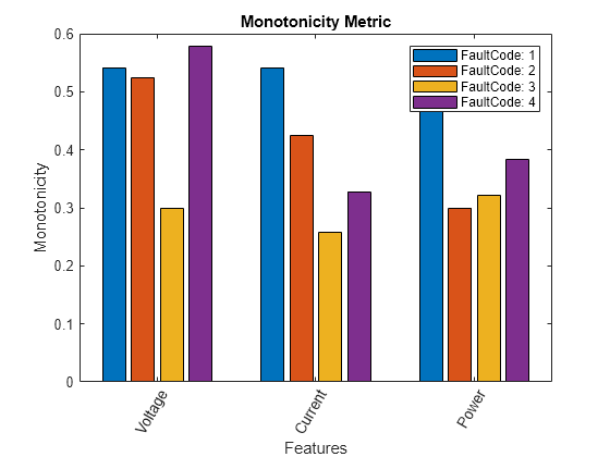
Visualize the monotonicity of the potential prognostic features with 'Machine' as the member variable and group the lifetime data by 'FaultCode'. Grouping the lifetime data ensures that monotonicity calculates the metric for each fault code separately.

monotonicity(ens,'MemberVariable','Machine','GroupBy','FaultCode');

Evaluating tall expression using the Local MATLAB Session:
- Pass 1 of 1: Completed in 0.42 sec
Evaluation completed in 0.87 sec
Evaluating tall expression using the Local MATLAB Session:
- Pass 1 of 1: Completed in 0.14 sec
Evaluation completed in 0.27 sec
Evaluating tall expression using the Local MATLAB Session:
- Pass 1 of 1: Completed in 0.35 sec
Evaluation completed in 0.39 sec

monotonicity returns a histogram plot with the features ranked by their monotonicity values. A higher monotonicity value indicates a more suitable prognostic parameter. For instance, the candidate feature Current has the highest monotonic trend for machines with FaultCode 1.

References

[1] Coble, J., and J. W. Hines. "Identifying Optimal Prognostic Parameters from Data: A Genetic Algorithms Approach." In Proceedings of the Annual Conference of the Prognostics and Health Management Society. 2009.
[2] Coble, J. "Merging Data Sources to Predict Remaining Useful Life - An Automated Method to Identify Prognostics Parameters." Ph.D. Thesis. University of Tennessee, Knoxville, TN, 2010.
[3] Lei, Y. Intelligent Fault Diagnosis and Remaining Useful Life Prediction of Rotating Machinery. Xi'an, China: Xi'an Jiaotong University Press, 2017.
[4] Lofti, S., J. B. Ali, E. Bechhoefer, and M. Benbouzid. "Wind turbine high-speed shaft bearings health prognosis through a spectral Kurtosis-derived indices and SVR." Applied Acoustics Vol. 120, 2017, pp. 1-8.
Version History
Introduced in R2018b