Explore Ensemble Data and Compare Features Using Diagnostic Feature Designer
The Diagnostic Feature Designer app allows you to accomplish the feature design portion of the predictive maintenance workflow using a multifunction graphical interface. You can design and compare features interactively and then determine which features are best at discriminating between data from different groups, such as nominal systems and faulty systems. If you have run-to-failure data, you can also evaluate which features are best for determining remaining useful life (RUL). The most effective features can ultimately become your condition indicators for fault diagnosis and prognostics.
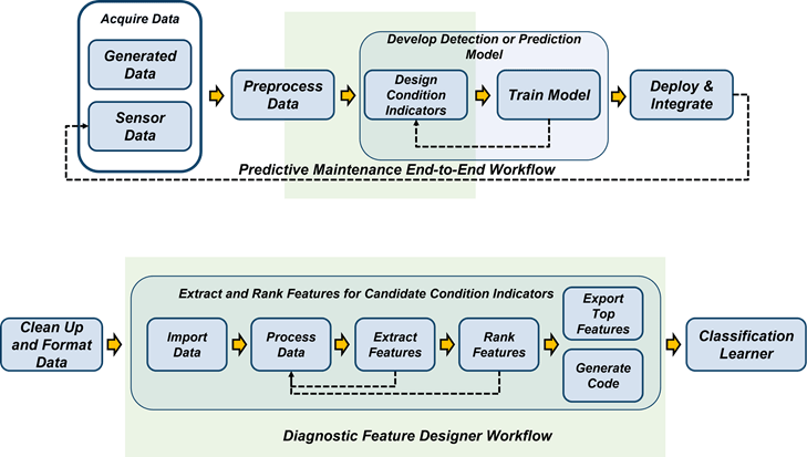
The following figure illustrates the relationship between the predictive maintenance workflow and Diagnostic Feature Designer functions.
The overall predictive maintenance workflow includes data acquisition, data preprocessing, designing condition indicators, training a model, and deploying and integrating the model. For more information on this workflow, see What Is Predictive Maintenance?.
The Diagnostic Feature Designer portion of the workflow starts with data import and includes the iterative process of processing data and extracting and ranking features to develop an effective feature set. This workflow also includes code generation as well feature export to tools like Classification Learner and Regression Learner for model generation and comparison.
The app operates on ensemble data. Ensemble data contains data measurements from multiple members, such as from multiple similar machines or from a single machine whose data is segmented by time intervals such as days or years. The data can also include condition variables, which describe the fault condition or operating condition of the ensemble member. Often condition variables have defined values known as labels. For more information on data ensembles, see Data Ensembles for Condition Monitoring and Predictive Maintenance.
The in-app workflow starts at the point of data import with data that is already:
Preprocessed with cleanup functions
Organized into either individual data files or a single ensemble data file that contains or references all ensemble members
Within Diagnostic Feature Designer, the workflow includes the steps required to further process your data, extract features from your data, and rank those features by effectiveness. The workflow concludes with selecting the most effective features and exporting those features to the Classification Learner or Regression Learner app for model training.
The workflow includes an optional MATLAB® code generation step. When you generate code that captures the calculations for the features you choose, you can automate those calculations for a larger set of measurement data that includes more members, such as similar machines from different factories. The resulting feature set provides additional training inputs for Classification Learner and Regression Learner. You can also generate code or a Simulink® block that is formatted for streaming data.
Perform Predictive Maintenance Tasks with Diagnostic Feature Designer
The following image illustrates the basic functionalities of Diagnostic Feature Designer. Interact with your data and your results by using controls in tabs such as the Feature Designer tab, which is shown in the figure. View your imported and derived variables, features, and data sets in the Data Browser. Visualize your results in the plotting area.

Convert Imported Data into Unified Ensemble Data Set
The first step in using the app is to create a new session and import your data. You can import data from tables, timetables, cell arrays, or matrices. You can also import an ensemble datastore that contains information that allows the app to interact with external data files. Your files can contain actual or simulated time-domain measurement data, spectral models or data, variable names, condition and operational variables, and features you generated previously. Diagnostic Feature Designer combines all your member data into a single ensemble data set. In this data set, each variable is a collective signal or model that contains all the individual member values.
To use the same data in multiple sessions, you can save your initial session in a session file. The session data includes both imported variables and any additional variables and features you have computed. In a subsequent session, you can then open the session file and continue working with your imported and derived data.
For information on preparing and importing your data, see:
For information on the import process itself, see Import and Visualize Ensemble Data in Diagnostic Feature Designer.
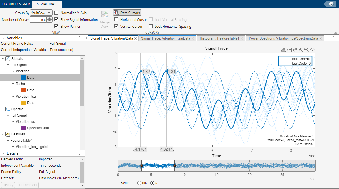
Visualize Data
To plot the signals or spectra that you import or that you generate with the processing tools, select a plot type from the plot gallery. The figure here illustrates a typical signal trace. Interactive plotting tools allow you to pan, zoom, display peak locations and distances between peaks, and show statistical variation within the ensemble. Grouping data by condition label in plots allows you to clearly see whether member data comes from, for example, nominal or faulty systems.
For information on plotting in the app, see Import and Visualize Ensemble Data in Diagnostic Feature Designer.
Compute New Variables
To explore your data and to prepare your data for feature extraction, use the data processing tools. Every time you apply a processing tool, the app creates a new derived variable with a name that contains both the source variable and the most recent processing step that you used. For example:
If you apply time-synchronous signal averaging (TSA) processing to the variable
Vibration/Data, the new derived variable name isVibration_tsa/Data.If you then compute a power spectrum from
Vibration_tsa/Data, the new variable name isVibration_ps/SpectrumData. This new name reflects both the most recent processingpsand the fact that the variable is a spectrum rather than a signal.
To obtain more information about a variable, use the Details pane. In this area, you can find information such as the direct source signal and the independent variable. You can also plot the processing history for the variable and view the parameters for the most recent operation.
Data processing options for all signals include ensemble-level statistics, signal residues, filtering, and power and order spectra. You can also interpolate your data to a uniform grid if your member samples do not occur at the same independent variable intervals.
If your data comes from rotating machinery, you can perform TSA processing based on your tachometer outputs or your nominal rpm. From the TSA signal, you can generate additional signals such as TSA residual and difference signals. These TSA-derived signals isolate physical components within your system by retaining or discarding harmonics and sidebands, and they are the basis for many of the gear condition features.
Many of the processing options can be used independently. Some options can or must be performed as a sequence. In addition to the rotating machinery and TSA signals previously discussed, another example is residue generation for any signal. You can:
Use Ensemble Statistics to generate single-member statistical variables such as mean and max that characterize the entire ensemble.
Use Subtract Reference to generate residue signals for each member by subtracting the ensemble-level values. These residues represent the variation among signals, and can more clearly reveal signals that deviate from the rest of the ensemble.
Use these residual signals as the source for additional processing options or for feature generation.
For information on data processing options in the app, see Process Data and Explore Features in Diagnostic Feature Designer.
Frame-Based and Parallel Processing
The app provides options for frame-based (segmented) and parallel processing.
By default, the app processes your entire signal in one operation. You can also segment the signals and process the individual frames. Frame-based processing is particularly useful if the members in your ensemble exhibit nonstationary, time-varying, or periodic behavior. Frame-based processing also supports prognostic ranking, since it provides a time history of feature values.
If you have Parallel Computing Toolbox™, you can use parallel processing. Because the app often performs the same processing independently on all members, parallel processing can significantly improve computation time.
Generate Features
From your original and derived signals and spectra, you can compute features and assess their effectiveness. You might already know which features are likely to work best, or you might want to experiment with all the applicable features. Available features range from general signal statistics, to specialized gear condition metrics that can identify the precise location of faults, to nonlinear features that highlight chaotic behavior.
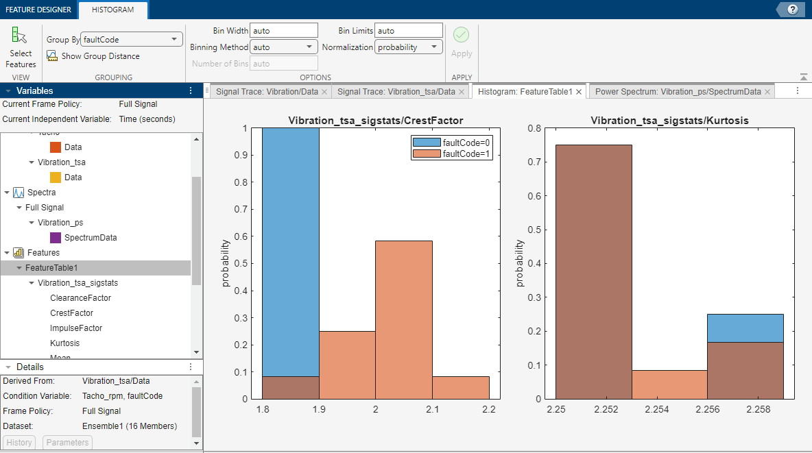
Any time you compute a set of features, the app adds them to the feature table and
generates a histogram of the distribution of values across the members. The figure here
illustrates histograms for two features. The histograms illustrate how well each feature
differentiates labeled data. For example, suppose that your condition variable is
faultCode with states 0 (color blue) for
nominal-system data and 1 (color orange) for faulty-system data, as shown
in the following figure. You can see in the histogram whether the nominal and faulty
groupings result in distinct or intermixed histogram bins by the presence of color mixing
within the bins. You can view all the feature histograms at once or select which features
the app includes in the histogram plot set. In the figure, the
CrestFactor bins are either primarily pure blue or pure orange, which
indicates good differentiation. The Kurtosis histogram bins are primarily
a dark orange that is a mix between blue and orange, indicating poor differentiation.
To compare the values of all your features together, use the feature table view and the feature trace plot. The feature table view displays a table of all the feature values of all the ensemble members. The feature trace plots these values. This plot visualizes the divergence of feature values within your ensemble and allows you to identify the specific member that a feature value represents.
For information on feature generation and histogram interpretation in the app, see:
Rank Features
Histograms allow you to perform an initial assessment of feature effectiveness. To perform a more rigorous relative assessment, you can rank your features using specialized statistical methods. The app provides three types of ranking: supervised ranking, unsupervised ranking, and prognostic ranking.
Supervised ranking includes methods for both classification ranking and regression ranking.
Classification ranking scores and ranks features by their ability to discriminate between or among data groups, such as between nominal and faulty behavior. This type of ranking requires condition variables that contain the labels that characterize the data groups.
Regression ranking scores and ranks features by their ability to predict numeric responses accurately. This type of ranking requires condition variables that provide the actual numeric responses.
Unsupervised ranking does not require condition variables such as data labels or response data. This type of ranking scores and ranks features based on their tendency to cluster with other features.
Prognostic ranking methods score and rank features based on the ability to track degradation in order to enable prediction of remaining useful life (RUL). Prognostic ranking requires real or simulated run-to-failure or fault-progression data and does not use condition variables.
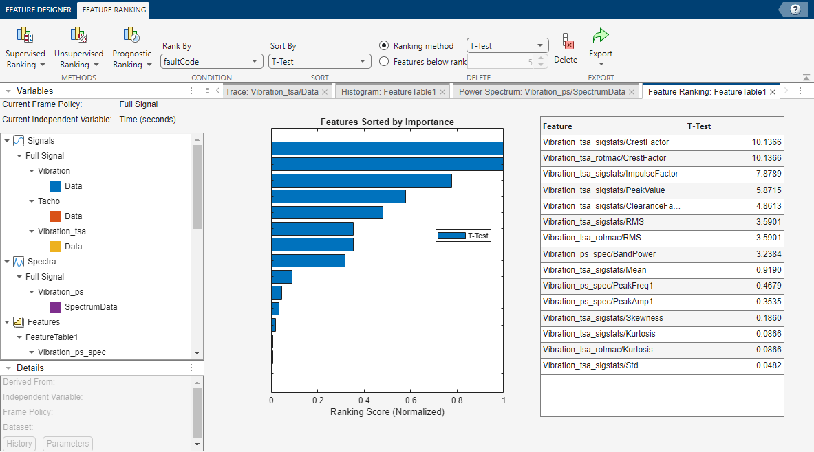
The following figure illustrates supervised classification ranking results. You can try multiple ranking methods and view the results from each method together. The ranking results allow you to eliminate ineffective features and to evaluate the ranking effects of parameter adjustments when computing derived variables or features.
For information on feature ranking, see:
Diagnostic Feature Designer sections for Feature Ranking Tab and Ranking Technique
Perform Prognostic Feature Ranking for a Degrading System Using Diagnostic Feature Designer
Export Features
After you have defined your set of candidate features, you can export them to the Classification Learner or Regression Learner app in the Statistics and Machine Learning Toolbox™.
Classification Learner trains models to classify data by using automated methods to test different types of models with a feature set. In doing so, Classification Learner determines the best model and the most effective features. For predictive maintenance, the goal of using Classification Learner is to select and train a model that discriminates between data from healthy and from faulty systems. You can incorporate this model into an algorithm for fault detection and prediction. For an example of exporting from the app into Classification Learner, see Analyze and Select Features for Pump Diagnostics.
Regression Learner trains models to predict numeric responses, also by using automated methods to find the best model and most effective features. You can incorporate this model into an algorithm for fault detection and prediction that includes thresholds that indicate when the predicted responses break operational limits.
You can also export your features and data sets to the MATLAB workspace. Doing so allows you to visualize and process your original and derived ensemble data using command-line functions or other apps. At the command line, you can also save features and variables that you select into files, including files referenced in an ensemble datastore.
For information on export, see Rank and Export Features in Diagnostic Feature Designer.
Generate MATLAB Code for Your Features
In addition to exporting the features themselves, you can generate a MATLAB function that reproduces the computations that created those features. Generating code allows you to automate the feature computations with different data sets. For instance, suppose you have a large input data set with many members, but for faster app response, you want to use a subset of that data when you first explore possible features interactively. After you identify your most effective features using the app, you can generate code and then use that code to apply the same feature computations to the all-member data set. The larger member set lets you provide more samples as training inputs to Classification Learner.
The following figure illustrates the Code Generation tab, which allows you to perform a detailed query to select features based on criteria such as feature input and computation method.
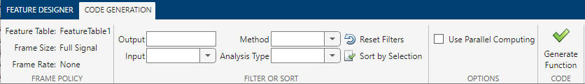
function [featureTable,outputTable] = diagnosticFeatures(inputData)
%DIAGNOSTICFEATURES recreates results in Diagnostic Feature Designer.
%
You can also generate code that is formatted for streaming data as well as a Simulink block that uses that code.
For more information, see:
See Also
See Also
Topics
- Isolate a Shaft Fault Using Diagnostic Feature Designer
- Design Condition Indicators for Predictive Maintenance Algorithms
- Organize System Data for Diagnostic Feature Designer
- Import Data into Diagnostic Feature Designer
- Data Preprocessing for Condition Monitoring and Predictive Maintenance
- Condition Indicators for Monitoring, Fault Detection, and Prediction