lasso

Lasso or elastic net regularization for linear models

Syntax

B = lasso(X,y)

B = lasso(X,y,Name=Value)

[B,FitInfo]
= lasso(___)

Description

B = lasso(X,y) returns fitted least-squares regression coefficients for linear models of the predictor data X and the response y. Each column of B corresponds to a particular regularization coefficient in Lambda. By default, lasso performs lasso regularization using a geometric sequence of Lambda values.

example

B = lasso(X,y,Name=Value) fits regularized regressions with additional options specified by one or more name-value pair arguments. For example, Alpha=0.5 sets elastic net as the regularization method, with the parameter Alpha equal to 0.5.

example

[B,FitInfo] = lasso(___) also returns the structure FitInfo, which contains information about the fit of the models, using any of the input arguments in the previous syntaxes.

example

Examples

collapse all

Remove Redundant Predictors Using Lasso Regularization

Open Live Script

Construct a data set with redundant predictors and identify those predictors by using lasso.

Create a matrix X of 100 five-dimensional normal variables. Create a response vector y from just two components of X, and add a small amount of noise.

rng default % For reproducibility
X = randn(100,5);
weights = [0;2;0;-3;0]; % Only two nonzero coefficients
y = X*weights + randn(100,1)*0.1; % Small added noise

Construct the default lasso fit.

B = lasso(X,y);

Find the coefficient vector for the 25th Lambda value in B.

B(:,25)

lasso identifies and removes the redundant predictors.

Create Linear Model Without Intercept Term Using Lasso Regularization

Open Live Script

Create sample data with predictor variable X and response variable $y = 0 + 2 X + ε$ .

rng default %   For reproducibility
X = rand(100,1);
y = 2*X + randn(100,1)/10;

Specify a regularization value, and find the coefficient of the regression model without an intercept term.

lambda = 1e-03;
B = lasso(X,y,Lambda=lambda,Intercept=false)

Warning: When the 'Intercept' value is false, the 'Standardize' value is set to false.

B = 
1.9825

Plot the real values (points) against the predicted values (line).

scatter(X,y)
hold on
x = 0:0.1:1;
plot(x,x*B)
hold off

Figure contains an axes object. The axes object contains 2 objects of type scatter, line.

Remove Redundant Predictors by Using Cross-Validated Fits

Open Live Script

Construct a data set with redundant predictors and identify those predictors by using cross-validated lasso.

Create a matrix X of 100 five-dimensional normal variables. Create a response vector y from two components of X, and add a small amount of noise.

rng default % For reproducibility
X = randn(100,5);
weights = [0;2;0;-3;0]; % Only two nonzero coefficients
y = X*weights + randn(100,1)*0.1; % Small added noise

Construct the lasso fit by using 10-fold cross-validation with labeled predictor variables.

[B,FitInfo] = lasso(X,y,CV=10,PredictorNames=["x1","x2","x3","x4","x5"]);

Display the variables in the model that corresponds to the minimum cross-validated mean squared error (MSE).

idxLambdaMinMSE = FitInfo.IndexMinMSE;
minMSEModelPredictors = FitInfo.PredictorNames(B(:,idxLambdaMinMSE)~=0)

minMSEModelPredictors = 1×2 cell
    {'x2'}    {'x4'}

Display the variables in the sparsest model within one standard error of the minimum MSE.

idxLambda1SE = FitInfo.Index1SE;
sparseModelPredictors = FitInfo.PredictorNames(B(:,idxLambda1SE)~=0)

sparseModelPredictors = 1×2 cell
    {'x2'}    {'x4'}

In this example, lasso identifies the same predictors for the two models and removes the redundant predictors.

Lasso Plot with Cross-Validated Fits

Open Live Script

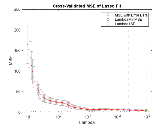
Visually examine the cross-validated error of various levels of regularization.

Load the sample data.

load acetylene

Create a design matrix with interactions and no constant term.

X = [x1 x2 x3];
D = x2fx(X,"interaction");
D(:,1) = []; % No constant term

Construct the lasso fit using 10-fold cross-validation. Include the FitInfo output so you can plot the result.

rng default % For reproducibility 
[B,FitInfo] = lasso(D,y,CV=10);

Plot the cross-validated fits. The green circle and dotted line locate the Lambda with minimum cross-validation error. The blue circle and dotted line locate the point with minimum cross-validation error plus one standard error.

lassoPlot(B,FitInfo,PlotType="CV");
legend("show")

Figure contains an axes object. The axes object with title Cross-Validated MSE of Lasso Fit, xlabel Lambda, ylabel MSE contains 5 objects of type errorbar, line. One or more of the lines displays its values using only markers These objects represent MSE with Error Bars, LambdaMinMSE, Lambda1SE.

Predict Values Using Elastic Net Regularization

Open Live Script

Predict students' exam scores using lasso and the elastic net method.

Load the examgrades data set.

load examgrades
X = grades(:,1:4);
y = grades(:,5);

Split the data into training and test sets.

n = length(y);
c = cvpartition(n,HoldOut=0.3);
idxTrain = training(c,1);
idxTest = ~idxTrain;
XTrain = X(idxTrain,:);
yTrain = y(idxTrain);
XTest = X(idxTest,:);
yTest = y(idxTest);

Find the coefficients of a regularized linear regression model using 10-fold cross-validation and the elastic net method with Alpha = 0.75. Use the largest Lambda value such that the mean squared error (MSE) is within one standard error of the minimum MSE.

[B,FitInfo] = lasso(XTrain,yTrain,Alpha=0.75,CV=10);
idxLambda1SE = FitInfo.Index1SE;
coef = B(:,idxLambda1SE);
coef0 = FitInfo.Intercept(idxLambda1SE);

Predict exam scores for the test data. Compare the predicted values to the actual exam grades using a reference line.

yhat = XTest*coef + coef0;
hold on
scatter(yTest,yhat)
plot(yTest,yTest)
xlabel("Actual Exam Grades")
ylabel("Predicted Exam Grades")
hold off

Figure contains an axes object. The axes object with xlabel Actual Exam Grades, ylabel Predicted Exam Grades contains 2 objects of type scatter, line.

Use Correlation Matrix for Fitting Lasso

Open Live Script

Create a matrix X of N p-dimensional normal variables, where N is large and p = 1000. Create a response vector y from the model y = beta0 + X*p, where beta0 is a constant, along with additive noise.

rng default % For reproducibility
N = 1e4; % Number of samples
p = 1e3; % Number of features
X = randn(N,p);
beta = randn(p,1); % Multiplicative coefficients
beta0 = randn; % Additive term
y = beta0 + X*beta + randn(N,1); % Last term is noise

Construct the default lasso fit. Time the creation.

B = lasso(X,y,UseCovariance=false); % Warm up lasso for reliable timing data
tic
B = lasso(X,y,UseCovariance=false);
timefalse = toc

timefalse = 
6.4392

Construct the lasso fit using the covariance matrix. Time the creation.

B2 = lasso(X,y,UseCovariance=true); % Warm up lasso for reliable timing data
tic
B2 = lasso(X,y,UseCovariance=true);
timetrue = toc

timetrue = 
0.4342

The fitting time with the covariance matrix is much less than the time without it. View the speedup factor that results from using the covariance matrix.

speedup = timefalse/timetrue

speedup = 
14.8314

Check that the returned coefficients B and B2 are similar.

norm(B-B2)/norm(B)

ans = 
5.2508e-15

The results are virtually identical.

Input Arguments

collapse all

`X` — Predictor data
numeric matrix

Predictor data, specified as a numeric matrix. Each row represents one observation, and each column represents one predictor variable.

Data Types: single | double

`y` — Response data
numeric vector

Response data, specified as a numeric vector. y has length n, where n is the number of rows of X. The response y(i) corresponds to the ith row of X.

Data Types: single | double

Name-Value Arguments

collapse all

Specify optional pairs of arguments as Name1=Value1,...,NameN=ValueN, where Name is the argument name and Value is the corresponding value. Name-value arguments must appear after other arguments, but the order of the pairs does not matter.

Before R2021a, use commas to separate each name and value, and enclose Name in quotes.

Example: lasso(X,y,Alpha=0.75,CV=10) performs elastic net regularization with 10-fold cross-validation. The Alpha=0.75 name-value pair argument sets the parameter used in the elastic net optimization.

`AbsTol` — Absolute error tolerance
`1e–4` (default) | positive scalar

Absolute error tolerance used to determine the convergence of the ADMM Algorithm, specified as a positive scalar. The algorithm converges when successive estimates of the coefficient vector differ by an amount less than AbsTol.

Note

This option applies only when you use lasso on tall arrays. See Extended Capabilities for more information.

Example: AbsTol=1e–3

Data Types: single | double

`Alpha` — Weight of lasso versus ridge optimization
`1` (default) | positive scalar

Weight of lasso (L¹) versus ridge (L²) optimization, specified as a positive scalar value in the interval (0,1]. The value Alpha = 1 represents lasso regression, Alpha close to 0 approaches ridge regression, and other values represent elastic net optimization. See Elastic Net.

Example: Alpha=0.5

Data Types: single | double

`B0` — Initial values for x-coefficients in ADMM Algorithm
vector of zeros (default) | numeric vector

Initial values for x-coefficients in ADMM Algorithm, specified as a numeric vector.

Note

This option applies only when you use lasso on tall arrays. See Extended Capabilities for more information.

Data Types: single | double

`CacheSize` — Size of covariance matrix in megabytes
`1000` (default) | positive scalar | `"maximal"`

Size of the covariance matrix in megabytes, specified as a positive scalar or "maximal". The lasso function can use a covariance matrix for fitting when the UseCovariance argument is true or "auto".

If UseCovariance is true or "auto" and CacheSize is "maximal", lasso can attempt to allocate a covariance matrix that exceeds the available memory. In this case, MATLAB^® issues an error.

Example: CacheSize="maximal"

Data Types: double | char | string

`CV` — Cross-validation specification for estimating mean squared error
`"resubstitution"` (default) | positive integer scalar | `cvpartition` object

Cross-validation specification for estimating the mean squared error (MSE), specified as one of the following:

"resubstitution" — lasso uses X and y to fit the model and to estimate the MSE without cross-validation.
Positive scalar integer K — lasso uses K-fold cross-validation.
cvpartition object cvp — lasso uses the cross-validation method expressed in cvp. You cannot use a 'leaveout' or custom 'holdout' partition with lasso.

Example: CV=3

`DFmax` — Maximum number of nonzero coefficients
`Inf` (default) | positive integer scalar

Maximum number of nonzero coefficients in the model, specified as a positive integer scalar. lasso returns results only for Lambda values that satisfy this criterion.

Example: DFmax=5

Data Types: single | double

`Intercept` — Flag for fitting the model with intercept term
`true` (default) | `false`

Flag for fitting the model with the intercept term, specified as either true or false. The default value is true, which indicates to include the intercept term in the model. If Intercept is false, then the returned intercept value is 0.

Example: Intercept=false

Data Types: logical

`Lambda` — Regularization coefficients
nonnegative vector

Regularization coefficients, specified as a vector of nonnegative values. See Lasso.

If you do not supply Lambda, then lasso calculates the largest value of Lambda that gives a nonnull model. In this case, LambdaRatio gives the ratio of the smallest to the largest value of the sequence, and NumLambda gives the length of the vector.
If you supply Lambda, then lasso ignores LambdaRatio and NumLambda.
If Standardize is true, then Lambda is the set of values used to fit the models with the X data standardized to have zero mean and a variance of one.

The default is a geometric sequence of NumLambda values, with only the largest value able to produce B = 0.

Example: Lambda=linspace(0,1)

Data Types: single | double

`LambdaRatio` — Ratio of smallest to largest `Lambda` values
`1e–4` (default) | positive scalar

Ratio of the smallest to the largest Lambda values when you do not supply Lambda, specified as a positive scalar.

If you set LambdaRatio = 0, then lasso generates a default sequence of Lambda values and replaces the smallest one with 0.

Example: LambdaRatio=1e–2

Data Types: single | double

`MaxIter` — Maximum number of iterations allowed
positive integer scalar

Maximum number of iterations allowed, specified as a positive integer scalar.

If the algorithm executes MaxIter iterations before reaching the convergence tolerance RelTol, then the function stops iterating and returns a warning message.

The function can return more than one warning when NumLambda is greater than 1.

Default values are 1e5 for standard data and 1e4 for tall arrays.

Example: MaxIter=1e3

Data Types: single | double

`MCReps` — Number of Monte Carlo repetitions for cross-validation
`1` (default) | positive integer scalar

Number of Monte Carlo repetitions for cross-validation, specified as a positive integer scalar.

If CV is "resubstitution" or a cvpartition of type "resubstitution", then MCReps must be 1.
If CV is a cvpartition of type "holdout", then MCReps must be greater than 1.
If CV is a custom cvpartition of type "kfold", then MCReps must be 1.

Example: MCReps=5

Data Types: single | double

`NumLambda` — Number of `Lambda` values
`100` (default) | positive integer scalar

Number of Lambda values lasso uses when you do not supply Lambda, specified as a positive integer scalar. lasso can return fewer than NumLambda fits if the residual error of the fits drops below a threshold fraction of the variance of y.

Example: NumLambda=50

Data Types: single | double

`Options` — Options for computing in parallel and setting random streams
structure

Options for computing in parallel and setting random streams, specified as a structure. Parallel computation is not used when CV is "resubstitution". Create the Options structure using statset. This table lists the option fields and their values.

Field Name Value Default

UseParallel Set this value to true to run computations in parallel. false

Field Name	Value	Default
`UseParallel`	Set this value to `true` to run computations in parallel.	`false`
`UseSubstreams`	Set this value to `true` to run computations in a reproducible manner. To compute reproducibly, set `Streams` to a type that allows substreams: `"mlfg6331_64"` or `"mrg32k3a"`.	`false`
`Streams`	Specify this value as a `RandStream` object or cell array of such objects. Use a single object except when the `UseParallel` value is `true` and the `UseSubstreams` value is `false`. In that case, use a cell array that has the same size as the parallel pool.	If you do not specify `Streams`, then `lasso` uses the default stream or streams.

UseSubstreams

Set this value to true to run computations in a reproducible manner.

To compute reproducibly, set Streams to a type that allows substreams: "mlfg6331_64" or "mrg32k3a".

false

Streams Specify this value as a RandStream object or cell array of such objects. Use a single object except when the UseParallel value is true and the UseSubstreams value is false. In that case, use a cell array that has the same size as the parallel pool. If you do not specify Streams, then lasso uses the default stream or streams.

Note

You need Parallel Computing Toolbox™ to run computations in parallel.

Example: Options=statset(UseParallel=true,UseSubstreams=true,Streams=RandStream("mlfg6331_64"))

Data Types: struct

`PredictorNames` — Names of predictor variables
`{}` (default) | string array | cell array of character vectors

Names of the predictor variables, in the order in which they appear in X, specified as a string array or cell array of character vectors.

Example: PredictorNames=["x1","x2","x3","x4"]

Data Types: string | cell

`RelTol` — Convergence threshold for coordinate descent algorithm
`1e–4` (default) | positive scalar

Convergence threshold for the coordinate descent algorithm [3], specified as a positive scalar. The algorithm terminates when successive estimates of the coefficient vector differ in the L² norm by a relative amount less than RelTol.

Example: RelTol=5e–3

Data Types: single | double

`Rho` — Augmented Lagrangian parameter
positive scalar

Augmented Lagrangian parameter ρ for the ADMM Algorithm, specified as a positive scalar. The default is automatic selection.

Note

This option applies only when you use lasso on tall arrays. See Extended Capabilities for more information.

Example: Rho=2

Data Types: single | double

`Standardize` — Flag for standardizing predictor data before fitting models
`true` (default) | `false`

Flag for standardizing the predictor data X before fitting the models, either true or false. If Standardize is true, then the X data is scaled to have zero mean and a variance of one. Standardize affects whether the regularization is applied to the coefficients on the standardized scale or the original scale. The results are always presented on the original data scale.

If Intercept is false, then the software sets Standardize to false, regardless of the Standardize value you specify.

X and y are always centered when Intercept is true.

Example: Standardize=false

Data Types: logical

`UseCovariance` — Indication to use covariance matrix for fitting
`"auto"` (default) | logical scalar

Indication to use a covariance matrix for fitting, specified as "auto" or a logical scalar.

"auto" causes lasso to attempt to use a covariance matrix for fitting when the number of observations is greater than the number of problem variables. This attempt can fail when memory is insufficient. To find out whether lasso used a covariance matrix for fitting, examine the UseCovariance field of the FitInfo output.
true causes lasso to use a covariance matrix for fitting as long as the required size does not exceed CacheSize. If the required covariance matrix size exceeds CacheSize, lasso issues a warning and does not use a covariance matrix for fitting.
false causes lasso not to use a covariance matrix for fitting.

Using a covariance matrix for fitting can be faster than not using one, but can require more memory. See Use Correlation Matrix for Fitting Lasso. The speed increase can negatively affect numerical stability. For details, see Coordinate Descent Algorithm.

Example: UseCovariance=true

Data Types: logical | char | string

`U0` — Initial value of scaled dual variable
vector of zeros (default) | numeric vector

Initial value of the scaled dual variable u in the ADMM Algorithm, specified as a numeric vector.

Note

This option applies only when you use lasso on tall arrays. See Extended Capabilities for more information.

Data Types: single | double

`Weights` — Observation weights
`1/n*ones(n,1)` (default) | nonnegative vector

Observation weights, specified as a nonnegative vector. Weights has length n, where n is the number of rows of X. The lasso function scales Weights to sum to 1.

Data Types: single | double

Output Arguments

collapse all

`B` — Fitted coefficients
numeric matrix

Fitted coefficients, returned as a numeric matrix. B is a p-by-L matrix, where p is the number of predictors (columns) in X, and L is the number of Lambda values. You can specify the number of Lambda values using the NumLambda name-value pair argument.

The coefficient corresponding to the intercept term is a field in FitInfo.

Data Types: single | double

`FitInfo` — Fit information of models
structure

Fit information of the linear models, returned as a structure with the fields described in this table.

Field in `FitInfo`	Description
`Intercept`	Intercept term β₀ for each linear model, a `1`-by-L vector
`Lambda`	Lambda parameters in ascending order, a `1`-by-L vector
`Alpha`	Value of the `Alpha` parameter, a scalar
`DF`	Number of nonzero coefficients in `B` for each value of `Lambda`, a `1`-by-L vector
`MSE`	Mean squared error (MSE), a `1`-by-L vector
`PredictorNames`	Value of the `PredictorNames` parameter, stored as a cell array of character vectors
`UseCovariance`	Logical value indicating whether the covariance matrix was used in fitting. If the covariance was computed and used, this field is `true`. Otherwise, this field is `false`.

If CV is a cvpartition object, the FitInfo contains these additional fields.

Field in `FitInfo`	Description
`SE`	Standard error of MSE for each `Lambda`, as calculated during cross-validation, a `1`-by-L vector
`LambdaMinMSE`	`Lambda` value with the minimum MSE, a scalar
`Lambda1SE`	Largest `Lambda` value such that MSE is within one standard error of the minimum MSE, a scalar
`IndexMinMSE`	Index of `Lambda` with the value `LambdaMinMSE`, a scalar
`Index1SE`	Index of `Lambda` with the value `Lambda1SE`, a scalar

More About

collapse all

Lasso

For a given value of λ, a nonnegative parameter, lasso solves the problem

$\min_{β_{0}, β} (\frac{1}{2 N} \sum_{i = 1}^{N} {(y_{i} - β_{0} - x_{i}^{T} β)}^{2} + λ \sum_{j = 1}^{p} | β_{j} |) .$

N is the number of observations.
y_i is the response at observation i.
x_i is data, a vector of length p at observation i.
λ is a nonnegative regularization parameter corresponding to one value of Lambda.
The parameters β₀ and β are a scalar and a vector of length p, respectively.

As λ increases, the number of nonzero components of β decreases.

The lasso problem involves the L¹ norm of β, as contrasted with the elastic net algorithm.

Elastic Net

For α strictly between 0 and 1, and nonnegative λ, elastic net solves the problem

$\min_{β_{0}, β} (\frac{1}{2 N} \sum_{i = 1}^{N} {(y_{i} - β_{0} - x_{i}^{T} β)}^{2} + λ P_{α} (β)),$

where

$P_{α} (β) = \frac{(1 - α)}{2} {‖ β ‖}_{2}^{2} + α {‖ β ‖}_{1} = \sum_{j = 1}^{p} (\frac{(1 - α)}{2} β_{j}^{2} + α | β_{j} |) .$

Elastic net is the same as lasso when α = 1. For other values of α, the penalty term P_α(β) interpolates between the L¹ norm of β and the squared L² norm of β. As α shrinks toward 0, elastic net approaches ridge regression.

Algorithms

collapse all

Coordinate Descent Algorithm

lasso fits many values of λ simultaneously by an efficient procedure named coordinate descent, based on Friedman, Tibshirani, and Hastie [3]. The procedure has two main code paths depending on whether the fitting uses a covariance matrix. You can affect this choice with the UseCovariance name-value argument.

When lasso uses a covariance matrix to fit N data points and D predictors, the fitting has a rough computational complexity of D*D. Without a covariance matrix, the computational complexity is roughly N*D. So, typically, using a covariance matrix can be faster when N > D, and the default 'auto' setting of the UseCovariance argument makes this choice. Using a covariance matrix causes lasso to subtract larger numbers than otherwise, which can be less numerically stable. For details of the algorithmic differences, see [3]. For one comparison of timing and accuracy differences, see Use Correlation Matrix for Fitting Lasso.

ADMM Algorithm

When operating on tall arrays, lasso uses an algorithm based on the Alternating Direction Method of Multipliers (ADMM) [5]. The notation used here is the same as in the reference paper. This method solves problems of the form

Minimize $l (x) + g (z)$

Subject to $A x + B z = c$

Using this notation, the lasso regression problem is

Minimize $l (x) + g (z) = \frac{1}{2} {‖ A x - b ‖}_{2}^{2} + λ {‖ z ‖}_{1}$

Subject to $x - z = 0$

Because the loss function $l (x) = \frac{1}{2} {‖ A x - b ‖}_{2}^{2}$ is quadratic, the iterative updates performed by the algorithm amount to solving a linear system of equations with a single coefficient matrix but several right-hand sides. The updates performed by the algorithm during each iteration are

$\begin{array}{l} x^{k + 1} = {(A^{T} A + ρ I)}^{- 1} (A^{T} b + ρ (z^{k} - u^{k})) \\ z^{k + 1} = S_{λ / ρ} (x^{k + 1} + u^{k}) \\ u^{k + 1} = u^{k} + x^{k + 1} - z^{k + 1} \end{array}$

A is the dataset (a tall array), x contains the coefficients, ρ is the penalty parameter (augmented Lagrangian parameter), b is the response (a tall array), and S is the soft thresholding operator.

$S_{κ} (a) = {\begin{matrix} \begin{matrix} a - κ, & a > κ \end{matrix} \\ \begin{matrix} 0, & | a | \leq κ \end{matrix} \\ \begin{matrix} a + κ, & a < - κ \end{matrix} \end{matrix} .$

lasso solves the linear system using Cholesky factorization because the coefficient matrix $A^{T} A + ρ I$ is symmetric and positive definite. Because $ρ$ does not change between iterations, the Cholesky factorization is cached between iterations.

Even though A and b are tall arrays, they appear only in the terms $A^{T} A$ and $A^{T} b$ . The results of these two matrix multiplications are small enough to fit in memory, so they are precomputed and the iterative updates between iterations are performed entirely within memory.

References

[1] Tibshirani, R. “Regression Shrinkage and Selection via the Lasso.” Journal of the Royal Statistical Society. Series B, Vol. 58, No. 1, 1996, pp. 267–288.

[2] Zou, H., and T. Hastie. “Regularization and Variable Selection via the Elastic Net.” Journal of the Royal Statistical Society. Series B, Vol. 67, No. 2, 2005, pp. 301–320.

[3] Friedman, J., R. Tibshirani, and T. Hastie. “Regularization Paths for Generalized Linear Models via Coordinate Descent.” Journal of Statistical Software. Vol. 33, No. 1, 2010. https://www.jstatsoft.org/v33/i01

[4] Hastie, T., R. Tibshirani, and J. Friedman. The Elements of Statistical Learning. 2nd edition. New York: Springer, 2008.

[5] Boyd, S. “Distributed Optimization and Statistical Learning via the Alternating Direction Method of Multipliers.” Foundations and Trends in Machine Learning. Vol. 3, No. 1, 2010, pp. 1–122.

Extended Capabilities

expand all

Tall Arrays
Calculate with arrays that have more rows than fit in memory.

This function supports tall arrays for out-of-memory data with some limitations.

With tall arrays, lasso uses an algorithm based on ADMM (Alternating Direction Method of Multipliers).
No elastic net support. The Alpha parameter is always 1.
No cross-validation (CV name-value argument) support, which includes the related name-value argument MCReps.
The output FitInfo does not contain the additional fields 'SE', 'LambdaMinMSE', 'Lambda1SE', 'IndexMinMSE', and 'Index1SE'.
The Options name-value argument is not supported because it does not contain options that apply to the ADMM algorithm. You can tune the ADMM algorithm using name-value arguments.
Supported name-value arguments are:
- Lambda
- LambdaRatio
- NumLambda
- Standardize
- PredictorNames
- RelTol
- Weights
Additional name-value arguments to control the ADMM algorithm are:
- Rho — Augmented Lagrangian parameter, ρ. The default value is automatic selection.
- AbsTol — Absolute tolerance used to determine convergence. The default value is 1e–4.
- MaxIter — Maximum number of iterations. The default value is 1e4.
- B0 — Initial values for the coefficients x. The default value is a vector of zeros.
- U0 — Initial values of the scaled dual variable u. The default value is a vector of zeros.

For more information, see Tall Arrays.

Automatic Parallel Support
Accelerate code by automatically running computation in parallel using Parallel Computing Toolbox™.

To run in parallel, specify the Options name-value argument. Set the UseParallel field of the options structure to true using statset:

Options=statset(UseParallel=true)

Parallel computation is not used when CV is "resubstitution". For more information about parallel computing, see Run MATLAB Functions with Automatic Parallel Support (Parallel Computing Toolbox).

Version History

Introduced in R2011b

lasso

Syntax

Description

Examples

Remove Redundant Predictors Using Lasso Regularization

Create Linear Model Without Intercept Term Using Lasso Regularization

Remove Redundant Predictors by Using Cross-Validated Fits

Lasso Plot with Cross-Validated Fits

Predict Values Using Elastic Net Regularization

Use Correlation Matrix for Fitting Lasso

Input Arguments

X — Predictor data numeric matrix

y — Response data numeric vector

Name-Value Arguments

AbsTol — Absolute error tolerance 1e–4 (default) | positive scalar

Alpha — Weight of lasso versus ridge optimization 1 (default) | positive scalar

B0 — Initial values for x-coefficients in ADMM Algorithm vector of zeros (default) | numeric vector

CacheSize — Size of covariance matrix in megabytes 1000 (default) | positive scalar | "maximal"

CV — Cross-validation specification for estimating mean squared error "resubstitution" (default) | positive integer scalar | cvpartition object

DFmax — Maximum number of nonzero coefficients Inf (default) | positive integer scalar

Intercept — Flag for fitting the model with intercept term true (default) | false

Lambda — Regularization coefficients nonnegative vector

LambdaRatio — Ratio of smallest to largest Lambda values 1e–4 (default) | positive scalar

MaxIter — Maximum number of iterations allowed positive integer scalar

MCReps — Number of Monte Carlo repetitions for cross-validation 1 (default) | positive integer scalar

NumLambda — Number of Lambda values 100 (default) | positive integer scalar

Options — Options for computing in parallel and setting random streams structure

PredictorNames — Names of predictor variables {} (default) | string array | cell array of character vectors

RelTol — Convergence threshold for coordinate descent algorithm 1e–4 (default) | positive scalar

Rho — Augmented Lagrangian parameter positive scalar

Standardize — Flag for standardizing predictor data before fitting models true (default) | false

UseCovariance — Indication to use covariance matrix for fitting "auto" (default) | logical scalar

U0 — Initial value of scaled dual variable vector of zeros (default) | numeric vector

Weights — Observation weights 1/n*ones(n,1) (default) | nonnegative vector

Output Arguments

B — Fitted coefficients numeric matrix

FitInfo — Fit information of models structure

More About

Lasso

Elastic Net

Algorithms

Coordinate Descent Algorithm

ADMM Algorithm

References

Extended Capabilities

Tall Arrays Calculate with arrays that have more rows than fit in memory.

Automatic Parallel Support Accelerate code by automatically running computation in parallel using Parallel Computing Toolbox™.

Version History

See Also

Topics

`X` — Predictor data
numeric matrix

`y` — Response data
numeric vector

`AbsTol` — Absolute error tolerance
`1e–4` (default) | positive scalar

`Alpha` — Weight of lasso versus ridge optimization
`1` (default) | positive scalar

`B0` — Initial values for x-coefficients in ADMM Algorithm
vector of zeros (default) | numeric vector

`CacheSize` — Size of covariance matrix in megabytes
`1000` (default) | positive scalar | `"maximal"`

`CV` — Cross-validation specification for estimating mean squared error
`"resubstitution"` (default) | positive integer scalar | `cvpartition` object

`DFmax` — Maximum number of nonzero coefficients
`Inf` (default) | positive integer scalar

`Intercept` — Flag for fitting the model with intercept term
`true` (default) | `false`

`Lambda` — Regularization coefficients
nonnegative vector

`LambdaRatio` — Ratio of smallest to largest `Lambda` values
`1e–4` (default) | positive scalar

`MaxIter` — Maximum number of iterations allowed
positive integer scalar

`MCReps` — Number of Monte Carlo repetitions for cross-validation
`1` (default) | positive integer scalar

`NumLambda` — Number of `Lambda` values
`100` (default) | positive integer scalar

`Options` — Options for computing in parallel and setting random streams
structure

`PredictorNames` — Names of predictor variables
`{}` (default) | string array | cell array of character vectors

`RelTol` — Convergence threshold for coordinate descent algorithm
`1e–4` (default) | positive scalar

`Rho` — Augmented Lagrangian parameter
positive scalar

`Standardize` — Flag for standardizing predictor data before fitting models
`true` (default) | `false`

`UseCovariance` — Indication to use covariance matrix for fitting
`"auto"` (default) | logical scalar

`U0` — Initial value of scaled dual variable
vector of zeros (default) | numeric vector

`Weights` — Observation weights
`1/n*ones(n,1)` (default) | nonnegative vector

`B` — Fitted coefficients
numeric matrix

`FitInfo` — Fit information of models
structure

Tall Arrays
Calculate with arrays that have more rows than fit in memory.

Automatic Parallel Support
Accelerate code by automatically running computation in parallel using Parallel Computing Toolbox™.