Main Content

ridge

Ridge regression

Description

B = ridge(y,X,k) returns coefficient estimates for ridge regression models of the predictor data X and the response y. Each column of B corresponds to a particular ridge parameter k. By default, the function computes B after centering and scaling the predictors to have mean 0 and standard deviation 1. Because the model does not include a constant term, do not add a column of 1s to X.

example

B = ridge(y,X,k,scaled) specifies the scaling for the coefficient estimates in B. When scaled is 1 (default), ridge does not restore the coefficients to the original data scale. When scaled is 0, ridge restores the coefficients to the scale of the original data. For more information, see Coefficient Scaling.

example

Examples

collapse all

Perform ridge regression for a range of ridge parameters and observe how the coefficient estimates change.

Load the acetylene data set.

load acetylene

acetylene contains observations for the predictor variables x1, x2, and x3, and the response variable y.

Plot the predictor variables against each other. Observe any correlation between the variables.

plotmatrix([x1 x2 x3])

MATLAB figure

For example, note the linear correlation between x1 and x3.

Compute coefficient estimates for a multilinear model with interaction terms, for a range of ridge parameters. Use x2fx to create interaction terms and ridge to perform ridge regression.

X = [x1 x2 x3];
D = x2fx(X,'interaction');
D(:,1) = []; % No constant term
k = 0:1e-5:5e-3;
B = ridge(y,D,k);

Plot the ridge trace.

figure
plot(k,B,'LineWidth',2)
ylim([-100 100])
grid on 
xlabel('Ridge Parameter') 
ylabel('Standardized Coefficient') 
title('Ridge Trace') 
legend('x1','x2','x3','x1x2','x1x3','x2x3')

Figure contains an axes object. The axes object with title Ridge Trace, xlabel Ridge Parameter, ylabel Standardized Coefficient contains 6 objects of type line. These objects represent x1, x2, x3, x1x2, x1x3, x2x3.

The estimates stabilize to the right of the plot. Note that the coefficient of the x2x3 interaction term changes sign at a value of the ridge parameter 5*10-4.

Predict miles per gallon (MPG) values using ridge regression.

Load the carbig data set.

load carbig
X = [Acceleration Weight Displacement Horsepower];
y = MPG;

Split the data into training and test sets.

n = length(y);
rng('default') % For reproducibility
c = cvpartition(n,'HoldOut',0.3);
idxTrain = training(c,1);
idxTest = ~idxTrain;

Find the coefficients of a ridge regression model (with k = 5).

k = 5;
b = ridge(y(idxTrain),X(idxTrain,:),k,0);

Predict MPG values for the test data using the model.

yhat = b(1) + X(idxTest,:)*b(2:end);

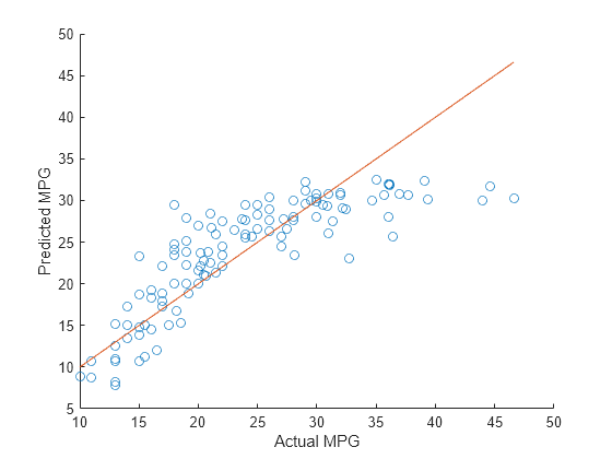
Compare the predicted values to the actual miles per gallon (MPG) values using a reference line.

scatter(y(idxTest),yhat)
hold on
plot(y(idxTest),y(idxTest))
xlabel('Actual MPG')
ylabel('Predicted MPG')
hold off

Figure contains an axes object. The axes object with xlabel Actual MPG, ylabel Predicted MPG contains 2 objects of type scatter, line.

Input Arguments

collapse all

Response data, specified as an n-by-1 numeric vector, where n is the number of observations.

Data Types: single | double

Predictor data, specified as an n-by-p numeric matrix. The rows of X correspond to the n observations, and the columns of X correspond to the p predictors.

Data Types: single | double

Ridge parameters, specified as a numeric vector.

Example: [0.2 0.3 0.4 0.5]

Data Types: single | double

Scaling flag that determines whether the coefficient estimates in B are restored to the scale of the original data, specified as either 0 or 1. If scaled is 0, then ridge performs this additional transformation. In this case, B contains p+1 coefficients for each value of k, with the first row of B corresponding to a constant term in the model. If scaled is 1, then the software omits the additional transformation, and B contains p coefficients without a constant term coefficient.

Output Arguments

collapse all

Coefficient estimates, returned as a numeric matrix. The rows of B correspond to the predictors in X, and the columns of B correspond to the ridge parameters k.

If scaled is 1, then B is a p-by-m matrix, where m is the number of elements in k. If scaled is 0, then B is a (p+1)-by-m matrix.

More About

collapse all

Ridge Regression

Ridge regression is a method for estimating coefficients of linear models that include linearly correlated predictors.

Coefficient estimates for multiple linear regression models rely on the independence of the model terms. When terms are correlated and the columns of the design matrix X have an approximate linear dependence, the matrix (XTX)–1 is close to singular. Therefore, the least-squares estimate

β^=(XTX)1XTy

is highly sensitive to random errors in the observed response y, producing a large variance. This situation of multicollinearity can arise, for example, when you collect data without an experimental design.

Ridge regression addresses the problem of multicollinearity by estimating regression coefficients using

β^=(XTX+kI)1XTy

where k is the ridge parameter and I is the identity matrix. Small, positive values of k improve the conditioning of the problem and reduce the variance of the estimates. While biased, the reduced variance of ridge estimates often results in a smaller mean squared error when compared to least-squares estimates.

Ridge Regularization

For a given value of λ, a nonnegative parameter, ridge solves the problem

minβ0,β(i=1N(yiβ0xiTβ)2+λj=1pβj2),

where:

  • N is the number of observations.

  • yi is the response at observation i.

  • xi is the data, a vector of length p at observation i.

  • λ is a nonnegative regularization parameter corresponding to one value of Lambda.

  • The parameter β0 is a scalar, and the parameter β is a vector of length p.

The lasso problem represents the L2 regularization element of Elastic Net.

Coefficient Scaling

The scaling of the coefficient estimates for the ridge regression models depends on the value of the scaled input argument.

Suppose the ridge parameter k is equal to 0. The coefficients returned by ridge, when scaled is equal to 1, are estimates of the bi1 in the multilinear model

yμy = b11z1 + ... + bp1zp + ε

where zi = (xiμi)/σi are the centered and scaled predictors, yμy is the centered response, and ε is an error term. You can rewrite the model as

y = b00 + b10x1 + ... + bp0xp + ε

with b00=μyi=1pbi1μiσi and bi0=bi1σi. The bi0 terms correspond to the coefficients returned by ridge when scaled is equal to 0.

More generally, for any value of k, if B1 = ridge(y,X,k,1), then

       m = mean(X);
       s = std(X,0,1)';
       B1_scaled = B1./s;
       B0 = [mean(y)-m*B1_scaled; B1_scaled]

where B0 = ridge(y,X,k,0).

Tips

  • ridge treats NaN values in X or y as missing values. ridge omits observations with missing values from the ridge regression fit.

  • In general, set scaled equal to 1 to produce plots where the coefficients are displayed on the same scale. See Ridge Regression for an example using a ridge trace plot, where the regression coefficients are displayed as a function of the ridge parameter. When making predictions, set scaled equal to 0. For an example, see Predict Values Using Ridge Regression.

Alternative Functionality

  • Ridge, lasso, and elastic net regularization are all methods for estimating the coefficients of a linear model while penalizing large coefficients. The type of penalty depends on the method (see More About for more details). To perform lasso or elastic net regularization, use lasso instead.

  • If you have high-dimensional full or sparse predictor data, you can use fitrlinear instead of ridge. When using fitrlinear, specify the 'Regularization','ridge' name-value pair argument. Set the value of the 'Lambda' name-value pair argument to a vector of the ridge parameters of your choice. fitrlinear returns a trained linear model Mdl. You can access the coefficient estimates stored in the Beta property of the model by using Mdl.Beta.

References

[1] Hoerl, A. E., and R. W. Kennard. “Ridge Regression: Biased Estimation for Nonorthogonal Problems.” Technometrics. Vol. 12, No. 1, 1970, pp. 55–67.

[2] Hoerl, A. E., and R. W. Kennard. “Ridge Regression: Applications to Nonorthogonal Problems.” Technometrics. Vol. 12, No. 1, 1970, pp. 69–82.

[3] Marquardt, D. W. “Generalized Inverses, Ridge Regression, Biased Linear Estimation, and Nonlinear Estimation.” Technometrics. Vol. 12, No. 3, 1970, pp. 591–612.

[4] Marquardt, D. W., and R. D. Snee. “Ridge Regression in Practice.” The American Statistician. Vol. 29, No. 1, 1975, pp. 3–20.

Version History

Introduced before R2006a