fitrlinear

Fit linear regression model to high-dimensional data

Syntax

Mdl = fitrlinear(X,Y)

Mdl = fitrlinear(Tbl,ResponseVarName)

Mdl = fitrlinear(Tbl,formula)

Mdl = fitrlinear(Tbl,Y)

Mdl = fitrlinear(X,Y,Name,Value)

[Mdl,FitInfo]
= fitrlinear(___)

[Mdl,FitInfo,HyperparameterOptimizationResults]
= fitrlinear(___)

Description

fitrlinear efficiently trains linear regression models with high-dimensional, full or sparse predictor data. Available linear regression models include regularized support vector machines (SVM) and least-squares regression methods. fitrlinear minimizes the objective function using techniques that reduce computing time (e.g., stochastic gradient descent).

For reduced computation time on a high-dimensional data set that includes many predictor variables, train a linear regression model by using fitrlinear. For low- through medium-dimensional predictor data sets, see Alternatives for Lower-Dimensional Data.

example

Mdl = fitrlinear(X,Y) returns a trained regression model object Mdl that contains the results of fitting a support vector machine regression model to the predictors X and response Y.

Mdl = fitrlinear(Tbl,ResponseVarName) returns a linear regression model using the predictor variables in the table Tbl and the response values in Tbl.ResponseVarName.

Mdl = fitrlinear(Tbl,formula) returns a linear regression model using the sample data in the table Tbl. The input argument formula is an explanatory model of the response and a subset of predictor variables in Tbl used to fit Mdl.

Mdl = fitrlinear(Tbl,Y) returns a linear regression model using the predictor variables in the table Tbl and the response values in vector Y.

example

Mdl = fitrlinear(X,Y,Name,Value) specifies options using one or more name-value pair arguments in addition to any of the input argument combinations in previous syntaxes. For example, you can specify to cross-validate, implement least-squares regression, or specify the type of regularization. A good practice is to cross-validate using the 'Kfold' name-value pair argument. The cross-validation results determine how well the model generalizes.

example

[Mdl,FitInfo] = fitrlinear(___) also returns optimization details using any of the previous syntaxes. You cannot request FitInfo for cross-validated models.

example

[Mdl,FitInfo,HyperparameterOptimizationResults] = fitrlinear(___) also returns hyperparameter optimization details when you pass an OptimizeHyperparameters name-value pair.

Examples

collapse all

Train Linear Regression Model

Open Live Script

Train a linear regression model using SVM, dual SGD, and ridge regularization.

Simulate 10000 observations from this model

$y = x_{100} + 2 x_{200} + e .$

$X = x_{1}, . . ., x_{1000}$ is a 10000-by-1000 sparse matrix with 10% nonzero standard normal elements.
e is random normal error with mean 0 and standard deviation 0.3.

rng(1) % For reproducibility
n = 1e4;
d = 1e3;
nz = 0.1;
X = sprandn(n,d,nz);
Y = X(:,100) + 2*X(:,200) + 0.3*randn(n,1);

Train a linear regression model. By default, fitrlinear uses support vector machines with a ridge penalty, and optimizes using dual SGD for SVM. Determine how well the optimization algorithm fit the model to the data by extracting a fit summary.

[Mdl,FitInfo] = fitrlinear(X,Y)

Mdl = 
  RegressionLinear
         ResponseName: 'Y'
    ResponseTransform: 'none'
                 Beta: [1000x1 double]
                 Bias: -0.0056
               Lambda: 1.0000e-04
              Learner: 'svm'


  Properties, Methods

FitInfo = struct with fields:
                    Lambda: 1.0000e-04
                 Objective: 0.2725
                 PassLimit: 10
                 NumPasses: 10
                BatchLimit: []
             NumIterations: 100000
              GradientNorm: NaN
         GradientTolerance: 0
      RelativeChangeInBeta: 0.4907
             BetaTolerance: 1.0000e-04
             DeltaGradient: 1.5816
    DeltaGradientTolerance: 0.1000
           TerminationCode: 0
         TerminationStatus: {'Iteration limit exceeded.'}
                     Alpha: [10000x1 double]
                   History: []
                   FitTime: 0.0679
                    Solver: {'dual'}

Mdl is a RegressionLinear model. You can pass Mdl and the training or new data to loss to inspect the in-sample mean-squared error. Or, you can pass Mdl and new predictor data to predict to predict responses for new observations.

FitInfo is a structure array containing, among other things, the termination status (TerminationStatus) and how long the solver took to fit the model to the data (FitTime). It is good practice to use FitInfo to determine whether optimization-termination measurements are satisfactory. In this case, fitrlinear reached the maximum number of iterations. Because training time is fast, you can retrain the model, but increase the number of passes through the data. Or, try another solver, such as LBFGS.

Find Good Lasso Penalty Using Cross-Validation

Open Live Script

To determine a good lasso-penalty strength for a linear regression model that uses least squares, implement 5-fold cross-validation.

Simulate 10000 observations from this model

$y = x_{100} + 2 x_{200} + e .$

$X = {x_{1}, . . ., x_{1000}}$ is a 10000-by-1000 sparse matrix with 10% nonzero standard normal elements.
e is random normal error with mean 0 and standard deviation 0.3.

rng(1) % For reproducibility
n = 1e4;
d = 1e3;
nz = 0.1;
X = sprandn(n,d,nz);
Y = X(:,100) + 2*X(:,200) + 0.3*randn(n,1);

Create a set of 15 logarithmically-spaced regularization strengths from $1 0^{- 5}$ through $1 0^{- 1}$ .

Lambda = logspace(-5,-1,15);

Cross-validate the models. To increase execution speed, transpose the predictor data and specify that the observations are in columns. Optimize the objective function using SpaRSA.

X = X'; 
CVMdl = fitrlinear(X,Y,'ObservationsIn','columns','KFold',5,'Lambda',Lambda,...
    'Learner','leastsquares','Solver','sparsa','Regularization','lasso');

numCLModels = numel(CVMdl.Trained)

numCLModels = 5

CVMdl is a RegressionPartitionedLinear model. Because fitrlinear implements 5-fold cross-validation, CVMdl contains 5 RegressionLinear models that the software trains on each fold.

Display the first trained linear regression model.

Mdl1 = CVMdl.Trained{1}

Mdl1 = 
  RegressionLinear
         ResponseName: 'Y'
    ResponseTransform: 'none'
                 Beta: [1000x15 double]
                 Bias: [1x15 double]
               Lambda: [1x15 double]
              Learner: 'leastsquares'


  Properties, Methods

Mdl1 is a RegressionLinear model object. fitrlinear constructed Mdl1 by training on the first four folds. Because Lambda is a sequence of regularization strengths, you can think of Mdl1 as 15 models, one for each regularization strength in Lambda.

Estimate the cross-validated MSE.

mse = kfoldLoss(CVMdl);

Higher values of Lambda lead to predictor variable sparsity, which is a good quality of a regression model. For each regularization strength, train a linear regression model using the entire data set and the same options as when you cross-validated the models. Determine the number of nonzero coefficients per model.

Mdl = fitrlinear(X,Y,'ObservationsIn','columns','Lambda',Lambda,...
    'Learner','leastsquares','Solver','sparsa','Regularization','lasso');
numNZCoeff = sum(Mdl.Beta~=0);

In the same figure, plot the cross-validated MSE and frequency of nonzero coefficients for each regularization strength. Plot all variables on the log scale.

figure
[h,hL1,hL2] = plotyy(log10(Lambda),log10(mse),...
    log10(Lambda),log10(numNZCoeff)); 
hL1.Marker = 'o';
hL2.Marker = 'o';
ylabel(h(1),'log_{10} MSE')
ylabel(h(2),'log_{10} nonzero-coefficient frequency')
xlabel('log_{10} Lambda')
hold off

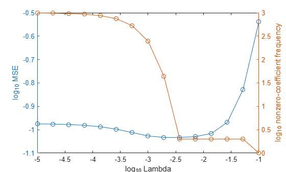
Choose the index of the regularization strength that balances predictor variable sparsity and low MSE (for example, Lambda(10)).

idxFinal = 10;

Extract the model with corresponding to the minimal MSE.

MdlFinal = selectModels(Mdl,idxFinal)

MdlFinal = 
  RegressionLinear
         ResponseName: 'Y'
    ResponseTransform: 'none'
                 Beta: [1000x1 double]
                 Bias: -0.0050
               Lambda: 0.0037
              Learner: 'leastsquares'


  Properties, Methods

idxNZCoeff = find(MdlFinal.Beta~=0)

idxNZCoeff = 2×1

   100
   200

EstCoeff = Mdl.Beta(idxNZCoeff)

EstCoeff = 2×1

    1.0051
    1.9965

MdlFinal is a RegressionLinear model with one regularization strength. The nonzero coefficients EstCoeff are close to the coefficients that simulated the data.

Optimize a Linear Regression

Open Live Script

This example shows how to optimize hyperparameters automatically using fitrlinear. The example uses artificial (simulated) data for the model

$y = x_{100} + 2 x_{200} + e .$

$X = {x_{1}, . . ., x_{1000}}$ is a 10000-by-1000 sparse matrix with 10% nonzero standard normal elements.
e is random normal error with mean 0 and standard deviation 0.3.

rng(1) % For reproducibility
n = 1e4;
d = 1e3;
nz = 0.1;
X = sprandn(n,d,nz);
Y = X(:,100) + 2*X(:,200) + 0.3*randn(n,1);

Find hyperparameters that minimize five-fold cross validation loss by using automatic hyperparameter optimization.

For reproducibility, use the 'expected-improvement-plus' acquisition function.

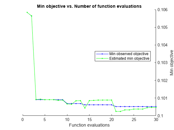
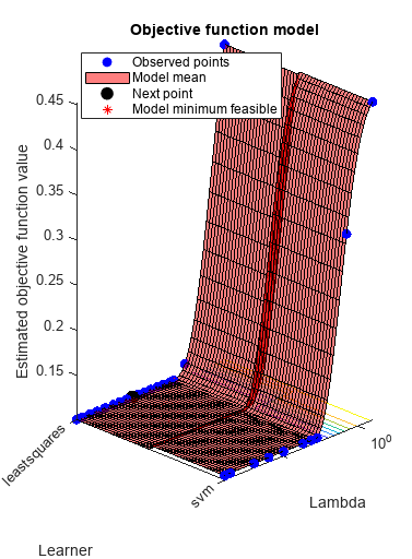
hyperopts = struct('AcquisitionFunctionName','expected-improvement-plus');
[Mdl,FitInfo,HyperparameterOptimizationResults] = fitrlinear(X,Y,...
    'OptimizeHyperparameters','auto',...
    'HyperparameterOptimizationOptions',hyperopts)

|=====================================================================================================|
| Iter | Eval   | Objective:  | Objective   | BestSoFar   | BestSoFar   |       Lambda |      Learner |
|      | result | log(1+loss) | runtime     | (observed)  | (estim.)    |              |              |
|=====================================================================================================|
|    1 | Best   |     0.16029 |     0.86667 |     0.16029 |     0.16029 |   2.4206e-09 |          svm |

|    2 | Best   |     0.14496 |     0.50145 |     0.14496 |     0.14601 |     0.001807 |          svm |

|    3 | Best   |     0.13879 |     0.41646 |     0.13879 |     0.14065 |   2.4681e-09 | leastsquares |

|    4 | Best   |       0.115 |     0.42001 |       0.115 |     0.11501 |     0.021027 | leastsquares |

|    5 | Accept |     0.44352 |     0.47308 |       0.115 |      0.1159 |       4.6795 | leastsquares |

|    6 | Best   |     0.11025 |     0.44839 |     0.11025 |     0.11024 |     0.010671 | leastsquares |

|    7 | Accept |     0.13222 |      0.3919 |     0.11025 |     0.11024 |   8.6067e-08 | leastsquares |

|    8 | Accept |     0.13262 |     0.43079 |     0.11025 |     0.11023 |   8.5109e-05 | leastsquares |

|    9 | Accept |     0.13543 |     0.40578 |     0.11025 |     0.11021 |   2.7562e-06 | leastsquares |

|   10 | Accept |     0.15751 |     0.44655 |     0.11025 |     0.11022 |   5.0559e-06 |          svm |

|   11 | Accept |     0.40673 |     0.40685 |     0.11025 |      0.1102 |      0.52074 |          svm |

|   12 | Accept |     0.16057 |     0.48935 |     0.11025 |      0.1102 |   0.00014292 |          svm |

|   13 | Accept |     0.16105 |     0.44932 |     0.11025 |     0.11018 |   1.0079e-07 |          svm |

|   14 | Accept |     0.12763 |     0.42144 |     0.11025 |     0.11019 |    0.0012085 | leastsquares |

|   15 | Accept |     0.13504 |     0.38616 |     0.11025 |     0.11019 |   1.3981e-08 | leastsquares |

|   16 | Accept |     0.11041 |     0.44711 |     0.11025 |     0.11026 |    0.0093968 | leastsquares |

|   17 | Best   |     0.10954 |      0.3604 |     0.10954 |     0.11003 |     0.010393 | leastsquares |

|   18 | Accept |     0.10998 |     0.32149 |     0.10954 |     0.11002 |     0.010254 | leastsquares |

|   19 | Accept |     0.45314 |     0.41668 |     0.10954 |     0.11001 |       9.9966 |          svm |

|   20 | Best   |     0.10753 |     0.45689 |     0.10753 |     0.10759 |     0.022576 |          svm |

|=====================================================================================================|
| Iter | Eval   | Objective:  | Objective   | BestSoFar   | BestSoFar   |       Lambda |      Learner |
|      | result | log(1+loss) | runtime     | (observed)  | (estim.)    |              |              |
|=====================================================================================================|
|   21 | Best   |     0.10737 |     0.44174 |     0.10737 |     0.10728 |     0.010171 |          svm |

|   22 | Accept |     0.13448 |     0.32469 |     0.10737 |     0.10727 |   1.5344e-05 | leastsquares |

|   23 | Best   |     0.10645 |     0.39821 |     0.10645 |     0.10565 |     0.015495 |          svm |

|   24 | Accept |     0.13598 |     0.32057 |     0.10645 |     0.10559 |   4.5984e-07 | leastsquares |

|   25 | Accept |     0.15962 |     0.42873 |     0.10645 |     0.10556 |   1.4302e-08 |          svm |

|   26 | Accept |     0.10689 |     0.43409 |     0.10645 |     0.10616 |     0.015391 |          svm |

|   27 | Accept |     0.13748 |     0.34492 |     0.10645 |     0.10614 |    1.001e-09 | leastsquares |

|   28 | Accept |     0.10692 |      0.3921 |     0.10645 |     0.10639 |     0.015761 |          svm |

|   29 | Accept |     0.10681 |     0.45101 |     0.10645 |     0.10649 |     0.015777 |          svm |

|   30 | Accept |     0.34314 |     0.34467 |     0.10645 |     0.10651 |      0.39671 | leastsquares |

__________________________________________________________
Optimization completed.
MaxObjectiveEvaluations of 30 reached.
Total function evaluations: 30
Total elapsed time: 47.3702 seconds
Total objective function evaluation time: 12.8375

Best observed feasible point:
     Lambda     Learner
    ________    _______

    0.015495      svm  

Observed objective function value = 0.10645
Estimated objective function value = 0.10651
Function evaluation time = 0.39821

Best estimated feasible point (according to models):
     Lambda     Learner
    ________    _______

    0.015777      svm  

Estimated objective function value = 0.10651
Estimated function evaluation time = 0.44103

Mdl = 
  RegressionLinear
         ResponseName: 'Y'
    ResponseTransform: 'none'
                 Beta: [1000x1 double]
                 Bias: -0.0018
               Lambda: 0.0158
              Learner: 'svm'


  Properties, Methods

FitInfo = struct with fields:
                    Lambda: 0.0158
                 Objective: 0.2309
                 PassLimit: 10
                 NumPasses: 10
                BatchLimit: []
             NumIterations: 99989
              GradientNorm: NaN
         GradientTolerance: 0
      RelativeChangeInBeta: 0.0641
             BetaTolerance: 1.0000e-04
             DeltaGradient: 1.1697
    DeltaGradientTolerance: 0.1000
           TerminationCode: 0
         TerminationStatus: {'Iteration limit exceeded.'}
                     Alpha: [10000x1 double]
                   History: []
                   FitTime: 0.0680
                    Solver: {'dual'}

HyperparameterOptimizationResults = 
  BayesianOptimization with properties:

                      ObjectiveFcn: @createObjFcn/inMemoryObjFcn
              VariableDescriptions: [3x1 optimizableVariable]
                           Options: [1x1 struct]
                      MinObjective: 0.1065
                   XAtMinObjective: [1x2 table]
             MinEstimatedObjective: 0.1065
          XAtMinEstimatedObjective: [1x2 table]
           NumObjectiveEvaluations: 30
                  TotalElapsedTime: 47.3702
                         NextPoint: [1x2 table]
                            XTrace: [30x2 table]
                    ObjectiveTrace: [30x1 double]
                  ConstraintsTrace: []
                     UserDataTrace: {30x1 cell}
      ObjectiveEvaluationTimeTrace: [30x1 double]
                IterationTimeTrace: [30x1 double]
                        ErrorTrace: [30x1 double]
                  FeasibilityTrace: [30x1 logical]
       FeasibilityProbabilityTrace: [30x1 double]
               IndexOfMinimumTrace: [30x1 double]
             ObjectiveMinimumTrace: [30x1 double]
    EstimatedObjectiveMinimumTrace: [30x1 double]

This optimization technique is simpler than that shown in Find Good Lasso Penalty Using Cross-Validation, but does not allow you to trade off model complexity and cross-validation loss.

Input Arguments

collapse all

`X` — Predictor data
full matrix | sparse matrix

Predictor data, specified as an n-by-p full or sparse matrix.

The length of Y and the number of observations in X must be equal.

Note

If you orient your predictor matrix so that observations correspond to columns and specify 'ObservationsIn','columns', then you might experience a significant reduction in optimization execution time.

Data Types: single | double

`Y` — Response data
numeric vector

Response data, specified as an n-dimensional numeric vector. The length of Y must be equal to the number of observations in X or Tbl.

Data Types: single | double

`Tbl` — Sample data
table

Sample data used to train the model, specified as a table. Each row of Tbl corresponds to one observation, and each column corresponds to one predictor variable. Optionally, Tbl can contain one additional column for the response variable. Multicolumn variables and cell arrays other than cell arrays of character vectors are not allowed.

If Tbl contains the response variable, and you want to use all remaining variables in Tbl as predictors, then specify the response variable by using ResponseVarName.

If Tbl contains the response variable, and you want to use only a subset of the remaining variables in Tbl as predictors, then specify a formula by using formula.

If Tbl does not contain the response variable, then specify a response variable by using Y. The length of the response variable and the number of rows in Tbl must be equal.

Data Types: table

`ResponseVarName` — Response variable name
name of variable in `Tbl`

Response variable name, specified as the name of a variable in Tbl. The response variable must be a numeric vector.

You must specify ResponseVarName as a character vector or string scalar. For example, if Tbl stores the response variable Y as Tbl.Y, then specify it as 'Y'. Otherwise, the software treats all columns of Tbl, including Y, as predictors when training the model.

Data Types: char | string

`formula` — Explanatory model of response variable and subset of predictor variables
character vector | string scalar

Explanatory model of the response variable and a subset of the predictor variables, specified as a character vector or string scalar in the form 'Y~X1+X2+X3'. In this form, Y represents the response variable, and X1, X2, and X3 represent the predictor variables.

To specify a subset of variables in Tbl as predictors for training the model, use a formula. If you specify a formula, then the software does not use any variables in Tbl that do not appear in formula.

The variable names in the formula must be both variable names in Tbl (Tbl.Properties.VariableNames) and valid MATLAB^® identifiers.

You can verify the variable names in Tbl by using the isvarname function. The following code returns logical 1 (true) for each variable that has a valid variable name.

cellfun(@isvarname,Tbl.Properties.VariableNames)

If the variable names in Tbl are not valid, then convert them by using the matlab.lang.makeValidName function.

Tbl.Properties.VariableNames = matlab.lang.makeValidName(Tbl.Properties.VariableNames);

Data Types: char | string

Note

The software treats NaN, empty character vector (''), empty string (""), <missing>, and <undefined> elements as missing values, and removes observations with any of these characteristics:

Missing value in the response (for example, Y or ValidationData{2})
At least one missing value in a predictor observation (for example, row in X or ValidationData{1})
NaN value or 0 weight (for example, value in Weights or ValidationData{3})

For memory-usage economy, it is best practice to remove observations containing missing values from your training data manually before training.

Name-Value Pair Arguments

Specify optional comma-separated pairs of Name,Value arguments. Name is the argument name and Value is the corresponding value. Name must appear inside quotes. You can specify several name and value pair arguments in any order as Name1,Value1,...,NameN,ValueN.

Example: Mdl = fitrlinear(X,Y,'Learner','leastsquares','CrossVal','on','Regularization','lasso') specifies to implement least-squares regression, implement 10-fold cross-validation, and specifies to include a lasso regularization term.

Note

You cannot use any cross-validation name-value pair argument along with the 'OptimizeHyperparameters' name-value pair argument. You can modify the cross-validation for 'OptimizeHyperparameters' only by using the 'HyperparameterOptimizationOptions' name-value pair argument.

Linear Regression Options

collapse all

`'Epsilon'` — Half the width of epsilon-insensitive band
`iqr(Y)/13.49` (default) | nonnegative scalar value

Half the width of the epsilon-insensitive band, specified as the comma-separated pair consisting of 'Epsilon' and a nonnegative scalar value. 'Epsilon' applies to SVM learners only.

The default Epsilon value is iqr(Y)/13.49, which is an estimate of standard deviation using the interquartile range of the response variable Y. If iqr(Y) is equal to zero, then the default Epsilon value is 0.1.

Example: 'Epsilon',0.3

Data Types: single | double

`'Lambda'` — Regularization term strength
`'auto'` (default) | nonnegative scalar | vector of nonnegative values

Regularization term strength, specified as the comma-separated pair consisting of 'Lambda' and 'auto', a nonnegative scalar, or a vector of nonnegative values.

For 'auto', Lambda = 1/n.
- If you specify a cross-validation, name-value pair argument (e.g., CrossVal), then n is the number of in-fold observations.
- Otherwise, n is the training sample size.
For a vector of nonnegative values, fitrlinear sequentially optimizes the objective function for each distinct value in Lambda in ascending order.
- If Solver is 'sgd' or 'asgd' and Regularization is 'lasso', fitrlinear does not use the previous coefficient estimates as a warm start for the next optimization iteration. Otherwise, fitrlinear uses warm starts.
- If Regularization is 'lasso', then any coefficient estimate of 0 retains its value when fitrlinear optimizes using subsequent values in Lambda.
- fitrlinear returns coefficient estimates for each specified regularization strength.

Example: 'Lambda',10.^(-(10:-2:2))

Data Types: char | string | double | single

`'Learner'` — Linear regression model type
`'svm'` (default) | `'leastsquares'`

Linear regression model type, specified as the comma-separated pair consisting of 'Learner' and 'svm' or 'leastsquares'.

In this table, $f (x) = x β + b .$

β is a vector of p coefficients.
x is an observation from p predictor variables.
b is the scalar bias.

Value	Algorithm	Response range	Loss function
`'leastsquares'`	Linear regression via ordinary least squares	y ∊ (-∞,∞)	Mean squared error (MSE): $ℓ [y, f (x)] = \frac{1}{2} {[y - f (x)]}^{2}$
`'svm'`	Support vector machine regression	Same as `'leastsquares'`	Epsilon-insensitive: $ℓ [y, f (x)] = \max [0, \| y - f (x) \| - ε]$

Example: 'Learner','leastsquares'

`'ObservationsIn'` — Predictor data observation dimension
`'rows'` (default) | `'columns'`

Predictor data observation dimension, specified as the comma-separated pair consisting of 'ObservationsIn' and 'columns' or 'rows'.

Note

`'Regularization'` — Complexity penalty type
`'lasso'` | `'ridge'`

Complexity penalty type, specified as the comma-separated pair consisting of 'Regularization' and 'lasso' or 'ridge'.

The software composes the objective function for minimization from the sum of the average loss function (see Learner) and the regularization term in this table.

Value	Description
`'lasso'`	Lasso (L1) penalty: $λ \sum_{j = 1}^{p} \| β_{j} \|$
`'ridge'`	Ridge (L2) penalty: $\frac{λ}{2} \sum_{j = 1}^{p} β_{j}^{2}$

To specify the regularization term strength, which is λ in the expressions, use Lambda.

The software excludes the bias term (β₀) from the regularization penalty.

If Solver is 'sparsa', then the default value of Regularization is 'lasso'. Otherwise, the default is 'ridge'.

Tip

For predictor variable selection, specify 'lasso'. For more on variable selection, see Introduction to Feature Selection.
For optimization accuracy, specify 'ridge'.

Example: 'Regularization','lasso'

`'Solver'` — Objective function minimization technique
`'sgd'` | `'asgd'` | `'dual'` | `'bfgs'` | `'lbfgs'` | `'sparsa'` | string array | cell array of character vectors

Objective function minimization technique, specified as the comma-separated pair consisting of 'Solver' and a character vector or string scalar, a string array, or a cell array of character vectors with values from this table.

Value	Description	Restrictions
`'sgd'`	Stochastic gradient descent (SGD) [5][3]
`'asgd'`	Average stochastic gradient descent (ASGD) [8]
`'dual'`	Dual SGD for SVM [2][7]	`Regularization` must be `'ridge'` and `Learner` must be `'svm'`.
`'bfgs'`	Broyden-Fletcher-Goldfarb-Shanno quasi-Newton algorithm (BFGS) [4]	Inefficient if `X` is very high-dimensional.
`'lbfgs'`	Limited-memory BFGS (LBFGS) [4]	`Regularization` must be `'ridge'`.
`'sparsa'`	Sparse Reconstruction by Separable Approximation (SpaRSA) [6]	`Regularization` must be `'lasso'`.

If you specify:

A ridge penalty (see Regularization) and size(X,1) <= 100 (100 or fewer predictor variables), then the default solver is 'bfgs'.
An SVM regression model (see Learner), a ridge penalty, and size(X,1) > 100 (more than 100 predictor variables), then the default solver is 'dual'.
A lasso penalty and X contains 100 or fewer predictor variables, then the default solver is 'sparsa'.

Otherwise, the default solver is 'sgd'.

If you specify a string array or cell array of solver names, then the software uses all solvers in the specified order for each Lambda.

For more details on which solver to choose, see Tips.

Example: 'Solver',{'sgd','lbfgs'}

`'Beta'` — Initial linear coefficient estimates
`zeros(p,1)` (default) | numeric vector | numeric matrix

Initial linear coefficient estimates (β), specified as the comma-separated pair consisting of 'Beta' and a p-dimensional numeric vector or a p-by-L numeric matrix. p is the number of predictor variables in X and L is the number of regularization-strength values (for more details, see Lambda).

If you specify a p-dimensional vector, then the software optimizes the objective function L times using this process.
1. The software optimizes using Beta as the initial value and the minimum value of Lambda as the regularization strength.
2. The software optimizes again using the resulting estimate from the previous optimization as a warm start, and the next smallest value in Lambda as the regularization strength.
3. The software implements step 2 until it exhausts all values in Lambda.
If you specify a p-by-L matrix, then the software optimizes the objective function L times. At iteration j, the software uses Beta(:,j) as the initial value and, after it sorts Lambda in ascending order, uses Lambda(j) as the regularization strength.

If you set 'Solver','dual', then the software ignores Beta.

Data Types: single | double

`'Bias'` — Initial intercept estimate
numeric scalar | numeric vector

Initial intercept estimate (b), specified as the comma-separated pair consisting of 'Bias' and a numeric scalar or an L-dimensional numeric vector. L is the number of regularization-strength values (for more details, see Lambda).

If you specify a scalar, then the software optimizes the objective function L times using this process.
1. The software optimizes using Bias as the initial value and the minimum value of Lambda as the regularization strength.
2. The uses the resulting estimate as a warm start to the next optimization iteration, and uses the next smallest value in Lambda as the regularization strength.
3. The software implements step 2 until it exhausts all values in Lambda.
If you specify an L-dimensional vector, then the software optimizes the objective function L times. At iteration j, the software uses Bias(j) as the initial value and, after it sorts Lambda in ascending order, uses Lambda(j) as the regularization strength.
By default:
- If Learner is 'leastsquares', then Bias is the weighted average of Y for training or, for cross-validation, in-fold responses.
- If Learner is 'svm', then Bias is the weighted median of Y for all training or, for cross-validation, in-fold observations that are greater than Epsilon.

Data Types: single | double

`'FitBias'` — Linear model intercept inclusion flag
`true` (default) | `false`

Linear model intercept inclusion flag, specified as the comma-separated pair consisting of 'FitBias' and true or false.

Value	Description
`true`	The software includes the bias term b in the linear model, and then estimates it.
`false`	The software sets b = 0 during estimation.

Example: 'FitBias',false

Data Types: logical

`'PostFitBias'` — Flag to fit linear model intercept after optimization
`false` (default) | `true`

Flag to fit the linear model intercept after optimization, specified as the comma-separated pair consisting of 'PostFitBias' and true or false.

Value Description

false The software estimates the bias term b and the coefficients β during optimization.

Value	Description
`false`	The software estimates the bias term b and the coefficients β during optimization.
`true`	To estimate b, the software: Estimates β and b using the model. Computes residuals. Refits b. For least squares, b is the weighted average of the residuals. For SVM regression, b is the weighted median between all residuals with magnitude greater than `Epsilon`.

true

To estimate b, the software:

Estimates β and b using the model.
Computes residuals.
Refits b. For least squares, b is the weighted average of the residuals. For SVM regression, b is the weighted median between all residuals with magnitude greater than Epsilon.

If you specify true, then FitBias must be true.

Example: 'PostFitBias',true

Data Types: logical

`'Verbose'` — Verbosity level
`0` (default) | nonnegative integer

Verbosity level, specified as the comma-separated pair consisting of 'Verbose' and a nonnegative integer. Verbose controls the amount of diagnostic information fitrlinear displays at the command line.

Value	Description
`0`	`fitrlinear` does not display diagnostic information.
`1`	`fitrlinear` periodically displays and stores the value of the objective function, gradient magnitude, and other diagnostic information. `FitInfo.History` contains the diagnostic information.
Any other positive integer	`fitrlinear` displays and stores diagnostic information at each optimization iteration. `FitInfo.History` contains the diagnostic information.

Example: 'Verbose',1

Data Types: double | single

SGD and ASGD Solver Options

collapse all

`'BatchSize'` — Mini-batch size
positive integer

Mini-batch size, specified as the comma-separated pair consisting of 'BatchSize' and a positive integer. At each iteration, the software estimates the subgradient using BatchSize observations from the training data.

If X is a numeric matrix, then the default value is 10.
If X is a sparse matrix, then the default value is max([10,ceil(sqrt(ff))]), where ff = numel(X)/nnz(X) (the fullness factor of X).

Example: 'BatchSize',100

Data Types: single | double

`'LearnRate'` — Learning rate
positive scalar

Learning rate, specified as the comma-separated pair consisting of 'LearnRate' and a positive scalar. LearnRate specifies how many steps to take per iteration. At each iteration, the gradient specifies the direction and magnitude of each step.

If Regularization is 'ridge', then LearnRate specifies the initial learning rate γ₀. The software determines the learning rate for iteration t, γ_t, using

$γ_{t} = \frac{γ_{0}}{{(1 + λ γ_{0} t)}^{c}} .$
- λ is the value of Lambda.
- If Solver is 'sgd', then c = 1.
- If Solver is 'asgd', then c is:
  - 2/3 if Learner is 'leastsquares'
  - 3/4 if Learner is 'svm' [8]
If Regularization is 'lasso', then, for all iterations, LearnRate is constant.

By default, LearnRate is 1/sqrt(1+max((sum(X.^2,obsDim)))), where obsDim is 1 if the observations compose the columns of X, and 2 otherwise.

Example: 'LearnRate',0.01

Data Types: single | double

`'OptimizeLearnRate'` — Flag to decrease learning rate
`true` (default) | `false`

Flag to decrease the learning rate when the software detects divergence (that is, over-stepping the minimum), specified as the comma-separated pair consisting of 'OptimizeLearnRate' and true or false.

If OptimizeLearnRate is 'true', then:

For the few optimization iterations, the software starts optimization using LearnRate as the learning rate.
If the value of the objective function increases, then the software restarts and uses half of the current value of the learning rate.
The software iterates step 2 until the objective function decreases.

Example: 'OptimizeLearnRate',true

Data Types: logical

`'TruncationPeriod'` — Number of mini-batches between lasso truncation runs
`10` (default) | positive integer

Number of mini-batches between lasso truncation runs, specified as the comma-separated pair consisting of 'TruncationPeriod' and a positive integer.

After a truncation run, the software applies a soft threshold to the linear coefficients. That is, after processing k = TruncationPeriod mini-batches, the software truncates the estimated coefficient j using

${\hat{β}}_{j}^{*} = {\begin{array}{l} {\hat{β}}_{j} - u_{t} & if {\hat{β}}_{j} > u_{t}, \\ 0 & if | {\hat{β}}_{j} | \leq u_{t}, \\ {\hat{β}}_{j} + u_{t} & if {\hat{β}}_{j} < - u_{t} . \end{array} \begin{array}{r} \end{array}$

For SGD, ${\hat{β}}_{j}$ is the estimate of coefficient j after processing k mini-batches. $u_{t} = k γ_{t} λ .$ γ_t is the learning rate at iteration t. λ is the value of Lambda.
For ASGD, ${\hat{β}}_{j}$ is the averaged estimate coefficient j after processing k mini-batches, $u_{t} = k λ .$

If Regularization is 'ridge', then the software ignores TruncationPeriod.

Example: 'TruncationPeriod',100

Data Types: single | double

Other Regression Options

collapse all

`'CategoricalPredictors'` — Categorical predictors list
vector of positive integers | logical vector | character matrix | string array | cell array of character vectors | `'all'`

Categorical predictors list, specified as the comma-separated pair consisting of 'CategoricalPredictors' and one of the values in this table. The descriptions assume that the predictor data has observations in rows and predictors in columns.

Value	Description
Vector of positive integers	Each entry in the vector is an index value corresponding to the column of the predictor data (`X` or `Tbl`) that contains a categorical variable.
Logical vector	A `true` entry means that the corresponding column of predictor data (`X` or `Tbl`) is a categorical variable.
Character matrix	Each row of the matrix is the name of a predictor variable. The names must match the entries in `PredictorNames`. Pad the names with extra blanks so each row of the character matrix has the same length.
String array or cell array of character vectors	Each element in the array is the name of a predictor variable. The names must match the entries in `PredictorNames`.
`'all'`	All predictors are categorical.

By default, if the predictor data is in a table (Tbl), fitrlinear assumes that a variable is categorical if it is a logical vector, categorical vector, character array, string array, or cell array of character vectors. If the predictor data is a matrix (X), fitrlinear assumes that all predictors are continuous. To identify any other predictors as categorical predictors, specify them by using the 'CategoricalPredictors' name-value pair argument.

For the identified categorical predictors, fitrlinear creates dummy variables using two different schemes, depending on whether a categorical variable is unordered or ordered. For an unordered categorical variable, fitrlinear creates one dummy variable for each level of the categorical variable. For an ordered categorical variable, fitrlinear creates one less dummy variable than the number of categories. For details, see Automatic Creation of Dummy Variables.

Example: 'CategoricalPredictors','all'

`'PredictorNames'` — Predictor variable names
string array of unique names | cell array of unique character vectors

Predictor variable names, specified as the comma-separated pair consisting of 'PredictorNames' and a string array of unique names or cell array of unique character vectors. The functionality of 'PredictorNames' depends on the way you supply the training data.

If you supply X and Y, then you can use 'PredictorNames' to assign names to the predictor variables in X.
- The order of the names in PredictorNames must correspond to the predictor order in X. Assuming that X has the default orientation, with observations in rows and predictors in columns, PredictorNames{1} is the name of X(:,1), PredictorNames{2} is the name of X(:,2), and so on. Also, size(X,2) and numel(PredictorNames) must be equal.
- By default, PredictorNames is {'x1','x2',...}.
If you supply Tbl, then you can use 'PredictorNames' to choose which predictor variables to use in training. That is, fitrlinear uses only the predictor variables in PredictorNames and the response variable during training.
- PredictorNames must be a subset of Tbl.Properties.VariableNames and cannot include the name of the response variable.
- By default, PredictorNames contains the names of all predictor variables.
- A good practice is to specify the predictors for training using either 'PredictorNames' or formula, but not both.

Example: 'PredictorNames',{'SepalLength','SepalWidth','PetalLength','PetalWidth'}

Data Types: string | cell

`'ResponseName'` — Response variable name
`'Y'` (default) | character vector | string scalar

Response variable name, specified as the comma-separated pair consisting of 'ResponseName' and a character vector or string scalar.

If you supply Y, then you can use 'ResponseName' to specify a name for the response variable.
If you supply ResponseVarName or formula, then you cannot use 'ResponseName'.

Example: 'ResponseName','response'

Data Types: char | string

`'ResponseTransform'` — Response transformation
`'none'` (default) | function handle

Response transformation, specified as the comma-separated pair consisting of 'ResponseTransform' and either 'none' or a function handle. The default is 'none', which means @(y)y, or no transformation. For a MATLAB function or a function you define, use its function handle. The function handle must accept a vector (the original response values) and return a vector of the same size (the transformed response values).

Example: Suppose you create a function handle that applies an exponential transformation to an input vector by using myfunction = @(y)exp(y). Then, you can specify the response transformation as 'ResponseTransform',myfunction.

Data Types: char | string | function_handle

`'Weights'` — Observation weights
positive numeric vector | name of variable in `Tbl`

Observation weights, specified as the comma-separated pair consisting of 'Weights' and a positive numeric vector or the name of a variable in Tbl. The software weights each observation in X or Tbl with the corresponding value in Weights. The length of Weights must equal the number of observations in X or Tbl.

If you specify the input data as a table Tbl, then Weights can be the name of a variable in Tbl that contains a numeric vector. In this case, you must specify Weights as a character vector or string scalar. For example, if weights vector W is stored as Tbl.W, then specify it as 'W'. Otherwise, the software treats all columns of Tbl, including W, as predictors when training the model.

By default, Weights is ones(n,1), where n is the number of observations in X or Tbl.

fitrlinear normalizes the weights to sum to 1.

Data Types: single | double | char | string

Cross-Validation Options

collapse all

`'CrossVal'` — Cross-validation flag
`'off'` (default) | `'on'`

Cross-validation flag, specified as the comma-separated pair consisting of 'Crossval' and 'on' or 'off'.

If you specify 'on', then the software implements 10-fold cross-validation.

To override this cross-validation setting, use one of these name-value pair arguments: CVPartition, Holdout, or KFold. To create a cross-validated model, you can use one cross-validation name-value pair argument at a time only.

Example: 'Crossval','on'

`'CVPartition'` — Cross-validation partition
`[]` (default) | `cvpartition` partition object

Cross-validation partition, specified as the comma-separated pair consisting of 'CVPartition' and a cvpartition partition object as created by cvpartition. The partition object specifies the type of cross-validation, and also the indexing for training and validation sets.

To create a cross-validated model, you can use one of these four options only: 'CVPartition', 'Holdout', or 'KFold'.

`'Holdout'` — Fraction of data for holdout validation
scalar value in the range (0,1)

Fraction of data used for holdout validation, specified as the comma-separated pair consisting of 'Holdout' and a scalar value in the range (0,1). If you specify 'Holdout',p, then the software:

Randomly reserves p*100% of the data as validation data, and trains the model using the rest of the data
Stores the compact, trained model in the Trained property of the cross-validated model.

To create a cross-validated model, you can use one of these four options only: 'CVPartition', 'Holdout', or 'KFold'.

Example: 'Holdout',0.1

Data Types: double | single

`'KFold'` — Number of folds
`10` (default) | positive integer value greater than 1

Number of folds to use in a cross-validated classifier, specified as the comma-separated pair consisting of 'KFold' and a positive integer value greater than 1. If you specify, e.g., 'KFold',k, then the software:

Randomly partitions the data into k sets
For each set, reserves the set as validation data, and trains the model using the other k – 1 sets
Stores the k compact, trained models in the cells of a k-by-1 cell vector in the Trained property of the cross-validated model.

To create a cross-validated model, you can use one of these four options only: 'CVPartition', 'Holdout', or 'KFold'.

Example: 'KFold',8

Data Types: single | double

SGD and ASGD Convergence Controls

collapse all

`'BatchLimit'` — Maximal number of batches
positive integer

Maximal number of batches to process, specified as the comma-separated pair consisting of 'BatchLimit' and a positive integer. When the software processes BatchLimit batches, it terminates optimization.

By default:
- The software passes through the data PassLimit times.
- If you specify multiple solvers, and use (A)SGD to get an initial approximation for the next solver, then the default value is ceil(1e6/BatchSize). BatchSize is the value of the 'BatchSize' name-value pair argument.
If you specify 'BatchLimit' and 'PassLimit', then the software chooses the argument that results in processing the fewest observations.
If you specify 'BatchLimit' but not 'PassLimit', then the software processes enough batches to complete up to one entire pass through the data.

Example: 'BatchLimit',100

Data Types: single | double

`'BetaTolerance'` — Relative tolerance on linear coefficients and bias term
`1e-4` (default) | nonnegative scalar

Relative tolerance on the linear coefficients and the bias term (intercept), specified as the comma-separated pair consisting of 'BetaTolerance' and a nonnegative scalar.

Let $B_{t} = [β_{t}^{'} b_{t}]$ , that is, the vector of the coefficients and the bias term at optimization iteration t. If ${‖ \frac{B_{t} - B_{t - 1}}{B_{t}} ‖}_{2} < BetaTolerance$ , then optimization terminates.

If the software converges for the last solver specified in Solver, then optimization terminates. Otherwise, the software uses the next solver specified in Solver.

Example: 'BetaTolerance',1e-6

Data Types: single | double

`'NumCheckConvergence'` — Number of batches to process before next convergence check
positive integer

Number of batches to process before next convergence check, specified as the comma-separated pair consisting of 'NumCheckConvergence' and a positive integer.

To specify the batch size, see BatchSize.

The software checks for convergence about 10 times per pass through the entire data set by default.

Example: 'NumCheckConvergence',100

Data Types: single | double

`'PassLimit'` — Maximal number of passes
`1` (default) | positive integer

Maximal number of passes through the data, specified as the comma-separated pair consisting of 'PassLimit' and a positive integer.

fitrlinear processes all observations when it completes one pass through the data.

When fitrlinear passes through the data PassLimit times, it terminates optimization.

If you specify 'BatchLimit' and PassLimit, then fitrlinear chooses the argument that results in processing the fewest observations. For more details, see Algorithms.

Example: 'PassLimit',5

Data Types: single | double

`'ValidationData'` — Validation data for optimization convergence detection
cell array | table

Validation data for optimization convergence detection, specified as the comma-separated pair consisting of 'ValidationData' and a cell array or table.

During optimization, the software periodically estimates the loss of ValidationData. If the validation-data loss increases, then the software terminates optimization. For more details, see Algorithms. To optimize hyperparameters using cross-validation, see cross-validation options such as CrossVal.

You can specify ValidationData as a table if you use a table Tbl of predictor data that contains the response variable. In this case, ValidationData must contain the same predictors and response contained in Tbl. The software does not apply weights to observations, even if Tbl contains a vector of weights. To specify weights, you must specify ValidationData as a cell array.

If you specify ValidationData as a cell array, then it must have the following format:

ValidationData{1} must have the same data type and orientation as the predictor data. That is, if you use a predictor matrix X, then ValidationData{1} must be an m-by-p or p-by-m full or sparse matrix of predictor data that has the same orientation as X. The predictor variables in the training data X and ValidationData{1} must correspond. Similarly, if you use a predictor table Tbl of predictor data, then ValidationData{1} must be a table containing the same predictor variables contained in Tbl. The number of observations in ValidationData{1} and the predictor data can vary.
ValidationData{2} must match the data type and format of the response variable, either Y or ResponseVarName. If ValidationData{2} is an array of responses, then it must have the same number of elements as the number of observations in ValidationData{1}. If ValidationData{1} is a table, then ValidationData{2} can be the name of the response variable in the table. If you want to use the same ResponseVarName or formula, you can specify ValidationData{2} as [].
Optionally, you can specify ValidationData{3} as an m-dimensional numeric vector of observation weights or the name of a variable in the table ValidationData{1} that contains observation weights. The software normalizes the weights with the validation data so that they sum to 1.

If you specify ValidationData and want to display the validation loss at the command line, specify a value larger than 0 for Verbose.

If the software converges for the last solver specified in Solver, then optimization terminates. Otherwise, the software uses the next solver specified in Solver.

By default, the software does not detect convergence by monitoring validation-data loss.

`'GradientTolerance'` — Absolute gradient tolerance
`1e-6` (default) | nonnegative scalar

Absolute gradient tolerance, specified as the comma-separated pair consisting of 'GradientTolerance' and a nonnegative scalar. GradientTolerance applies to these values of Solver: 'bfgs', 'lbfgs', and 'sparsa'.

Let $\nabla ℒ_{t}$ be the gradient vector of the objective function with respect to the coefficients and bias term at optimization iteration t. If ${‖ \nabla ℒ_{t} ‖}_{\infty} = \max | \nabla ℒ_{t} | < GradientTolerance$ , then optimization terminates.

If you also specify BetaTolerance, then optimization terminates when fitrlinear satisfies either stopping criterion.

If fitrlinear converges for the last solver specified in Solver, then optimization terminates. Otherwise, fitrlinear uses the next solver specified in Solver.

Example: 'GradientTolerance',eps

Data Types: single | double

`'IterationLimit'` — Maximal number of optimization iterations
`1000` (default) | positive integer

Maximal number of optimization iterations, specified as the comma-separated pair consisting of 'IterationLimit' and a positive integer. IterationLimit applies to these values of Solver: 'bfgs', 'lbfgs', and 'sparsa'.

Example: 'IterationLimit',1e7

Data Types: single | double

Dual SGD Optimization Convergence Controls

collapse all

`'BetaTolerance'` — Relative tolerance on linear coefficients and bias term
`1e-4` (default) | nonnegative scalar

Relative tolerance on the linear coefficients and the bias term (intercept), specified as the comma-separated pair consisting of 'BetaTolerance' and a nonnegative scalar.

If you also specify DeltaGradientTolerance, then optimization terminates when the software satisfies either stopping criterion.

If the software converges for the last solver specified in Solver, then optimization terminates. Otherwise, the software uses the next solver specified in Solver.

Example: 'BetaTolerance',1e-6

Data Types: single | double

`'DeltaGradientTolerance'` — Gradient-difference tolerance
`0.1` (default) | nonnegative scalar

Gradient-difference tolerance between upper and lower pool Karush-Kuhn-Tucker (KKT) complementarity conditions violators, specified as the comma-separated pair consisting of 'DeltaGradientTolerance' and a nonnegative scalar. DeltaGradientTolerance applies to the 'dual' value of Solver only.

If the magnitude of the KKT violators is less than DeltaGradientTolerance, then fitrlinear terminates optimization.
If fitrlinear converges for the last solver specified in Solver, then optimization terminates. Otherwise, fitrlinear uses the next solver specified in Solver.

Example: 'DeltaGapTolerance',1e-2

Data Types: double | single

`'NumCheckConvergence'` — Number of passes through entire data set to process before next convergence check
`5` (default) | positive integer

Number of passes through entire data set to process before next convergence check, specified as the comma-separated pair consisting of 'NumCheckConvergence' and a positive integer.

Example: 'NumCheckConvergence',100

Data Types: single | double

`'PassLimit'` — Maximal number of passes
`10` (default) | positive integer

Maximal number of passes through the data, specified as the comma-separated pair consisting of 'PassLimit' and a positive integer.

When the software completes one pass through the data, it has processed all observations.

When the software passes through the data PassLimit times, it terminates optimization.

Example: 'PassLimit',5

Data Types: single | double

`'ValidationData'` — Validation data for optimization convergence detection
cell array | table

Validation data for optimization convergence detection, specified as the comma-separated pair consisting of 'ValidationData' and a cell array or table.

If you specify ValidationData as a cell array, then it must have the following format:

ValidationData{1} must have the same data type and orientation as the predictor data. That is, if you use a predictor matrix X, then ValidationData{1} must be an m-by-p or p-by-m full or sparse matrix of predictor data that has the same orientation as X. The predictor variables in the training data X and ValidationData{1} must correspond. Similarly, if you use a predictor table Tbl of predictor data, then ValidationData{1} must be a table containing the same predictor variables contained in Tbl. The number of observations in ValidationData{1} and the predictor data can vary.
ValidationData{2} must match the data type and format of the response variable, either Y or ResponseVarName. If ValidationData{2} is an array of responses, then it must have the same number of elements as the number of observations in ValidationData{1}. If ValidationData{1} is a table, then ValidationData{2} can be the name of the response variable in the table. If you want to use the same ResponseVarName or formula, you can specify ValidationData{2} as [].
Optionally, you can specify ValidationData{3} as an m-dimensional numeric vector of observation weights or the name of a variable in the table ValidationData{1} that contains observation weights. The software normalizes the weights with the validation data so that they sum to 1.

If you specify ValidationData and want to display the validation loss at the command line, specify a value larger than 0 for Verbose.

If the software converges for the last solver specified in Solver, then optimization terminates. Otherwise, the software uses the next solver specified in Solver.

By default, the software does not detect convergence by monitoring validation-data loss.

BFGS, LBFGS, and SpaRSA Convergence Controls

collapse all

`'BetaTolerance'` — Relative tolerance on linear coefficients and bias term
`1e-4` (default) | nonnegative scalar

Relative tolerance on the linear coefficients and the bias term (intercept), specified as the comma-separated pair consisting of 'BetaTolerance' and a nonnegative scalar.

If you also specify GradientTolerance, then optimization terminates when the software satisfies either stopping criterion.

If the software converges for the last solver specified in Solver, then optimization terminates. Otherwise, the software uses the next solver specified in Solver.

Example: 'BetaTolerance',1e-6

Data Types: single | double

`'GradientTolerance'` — Absolute gradient tolerance
`1e-6` (default) | nonnegative scalar

Absolute gradient tolerance, specified as the comma-separated pair consisting of 'GradientTolerance' and a nonnegative scalar.

If you also specify BetaTolerance, then optimization terminates when the software satisfies either stopping criterion.

If the software converges for the last solver specified in the software, then optimization terminates. Otherwise, the software uses the next solver specified in Solver.

Example: 'GradientTolerance',1e-5

Data Types: single | double

`'HessianHistorySize'` — Size of history buffer for Hessian approximation
`15` (default) | positive integer

Size of history buffer for Hessian approximation, specified as the comma-separated pair consisting of 'HessianHistorySize' and a positive integer. That is, at each iteration, the software composes the Hessian using statistics from the latest HessianHistorySize iterations.

The software does not support 'HessianHistorySize' for SpaRSA.

Example: 'HessianHistorySize',10

Data Types: single | double

`'IterationLimit'` — Maximal number of optimization iterations
`1000` (default) | positive integer

Example: 'IterationLimit',500

Data Types: single | double

`'ValidationData'` — Validation data for optimization convergence detection
cell array | table

Validation data for optimization convergence detection, specified as the comma-separated pair consisting of 'ValidationData' and a cell array or table.

If you specify ValidationData as a cell array, then it must have the following format:

ValidationData{1} must have the same data type and orientation as the predictor data. That is, if you use a predictor matrix X, then ValidationData{1} must be an m-by-p or p-by-m full or sparse matrix of predictor data that has the same orientation as X. The predictor variables in the training data X and ValidationData{1} must correspond. Similarly, if you use a predictor table Tbl of predictor data, then ValidationData{1} must be a table containing the same predictor variables contained in Tbl. The number of observations in ValidationData{1} and the predictor data can vary.
ValidationData{2} must match the data type and format of the response variable, either Y or ResponseVarName. If ValidationData{2} is an array of responses, then it must have the same number of elements as the number of observations in ValidationData{1}. If ValidationData{1} is a table, then ValidationData{2} can be the name of the response variable in the table. If you want to use the same ResponseVarName or formula, you can specify ValidationData{2} as [].
Optionally, you can specify ValidationData{3} as an m-dimensional numeric vector of observation weights or the name of a variable in the table ValidationData{1} that contains observation weights. The software normalizes the weights with the validation data so that they sum to 1.

If you specify ValidationData and want to display the validation loss at the command line, specify a value larger than 0 for Verbose.

If the software converges for the last solver specified in Solver, then optimization terminates. Otherwise, the software uses the next solver specified in Solver.

By default, the software does not detect convergence by monitoring validation-data loss.

Hyperparameter Optimization

collapse all

`'OptimizeHyperparameters'` — Parameters to optimize
`'none'` (default) | `'auto'` | `'all'` | string array or cell array of eligible parameter names | vector of `optimizableVariable` objects

Parameters to optimize, specified as the comma-separated pair consisting of 'OptimizeHyperparameters' and one of the following:

'none' — Do not optimize.
'auto' — Use {'Lambda','Learner'}.
'all' — Optimize all eligible parameters.
String array or cell array of eligible parameter names.
Vector of optimizableVariable objects, typically the output of hyperparameters.

The optimization attempts to minimize the cross-validation loss (error) for fitrlinear by varying the parameters. To control the cross-validation type and other aspects of the optimization, use the HyperparameterOptimizationOptions name-value pair.

Note

'OptimizeHyperparameters' values override any values you set using other name-value pair arguments. For example, setting 'OptimizeHyperparameters' to 'auto' causes the 'auto' values to apply.

The eligible parameters for fitrlinear are:

Lambda — fitrlinear searches among positive values, by default log-scaled in the range [1e-5/NumObservations,1e5/NumObservations].
Learner — fitrlinear searches among 'svm' and 'leastsquares'.
Regularization — fitrlinear searches among 'ridge' and 'lasso'.

Set nondefault parameters by passing a vector of optimizableVariable objects that have nondefault values. For example,

load carsmall
params = hyperparameters('fitrlinear',[Horsepower,Weight],MPG);
params(1).Range = [1e-3,2e4];

Pass params as the value of OptimizeHyperparameters.

By default, iterative display appears at the command line, and plots appear according to the number of hyperparameters in the optimization. For the optimization and plots, the objective function is log(1 + cross-validation loss) for regression and the misclassification rate for classification. To control the iterative display, set the Verbose field of the 'HyperparameterOptimizationOptions' name-value pair argument. To control the plots, set the ShowPlots field of the 'HyperparameterOptimizationOptions' name-value pair argument.

For an example, see Optimize a Linear Regression.

Example: 'OptimizeHyperparameters','auto'

`'HyperparameterOptimizationOptions'` — Options for optimization
structure

Options for optimization, specified as the comma-separated pair consisting of 'HyperparameterOptimizationOptions' and a structure. This argument modifies the effect of the OptimizeHyperparameters name-value pair argument. All fields in the structure are optional.

Field Name	Values	Default
`Optimizer`	`'bayesopt'` — Use Bayesian optimization. Internally, this setting calls `bayesopt`. `'gridsearch'` — Use grid search with `NumGridDivisions` values per dimension. `'randomsearch'` — Search at random among `MaxObjectiveEvaluations` points. `'gridsearch'` searches in a random order, using uniform sampling without replacement from the grid. After optimization, you can get a table in grid order by using the command `sortrows(Mdl.HyperparameterOptimizationResults)`.	`'bayesopt'`
`AcquisitionFunctionName`	`'expected-improvement-per-second-plus'` `'expected-improvement'` `'expected-improvement-plus'` `'expected-improvement-per-second'` `'lower-confidence-bound'` `'probability-of-improvement'` Acquisition functions whose names include `per-second` do not yield reproducible results because the optimization depends on the runtime of the objective function. Acquisition functions whose names include `plus` modify their behavior when they are overexploiting an area. For more details, see Acquisition Function Types.	`'expected-improvement-per-second-plus'`
`MaxObjectiveEvaluations`	Maximum number of objective function evaluations.	`30` for `'bayesopt'` or `'randomsearch'`, and the entire grid for `'gridsearch'`
`MaxTime`	Time limit, specified as a positive real. The time limit is in seconds, as measured by `tic` and `toc`. Run time can exceed `MaxTime` because `MaxTime` does not interrupt function evaluations.	`Inf`
`NumGridDivisions`	For `'gridsearch'`, the number of values in each dimension. The value can be a vector of positive integers giving the number of values for each dimension, or a scalar that applies to all dimensions. This field is ignored for categorical variables.	`10`
`ShowPlots`	Logical value indicating whether to show plots. If `true`, this field plots the best objective function value against the iteration number. If there are one or two optimization parameters, and if `Optimizer` is `'bayesopt'`, then `ShowPlots` also plots a model of the objective function against the parameters.	`true`
`SaveIntermediateResults`	Logical value indicating whether to save results when `Optimizer` is `'bayesopt'`. If `true`, this field overwrites a workspace variable named `'BayesoptResults'` at each iteration. The variable is a `BayesianOptimization` object.	`false`
`Verbose`	Display to the command line. `0` — No iterative display `1` — Iterative display `2` — Iterative display with extra information For details, see the `bayesopt` `Verbose` name-value pair argument.	`1`
`UseParallel`	Logical value indicating whether to run Bayesian optimization in parallel, which requires Parallel Computing Toolbox™. Due to the nonreproducibility of parallel timing, parallel Bayesian optimization does not necessarily yield reproducible results. For details, see Parallel Bayesian Optimization.	`false`
`Repartition`	Logical value indicating whether to repartition the cross-validation at every iteration. If `false`, the optimizer uses a single partition for the optimization. `true` usually gives the most robust results because this setting takes partitioning noise into account. However, for good results, `true` requires at least twice as many function evaluations.	`false`
Use no more than one of the following three field names.
`CVPartition`	A `cvpartition` object, as created by `cvpartition`.	`'Kfold',5` if you do not specify any cross-validation field
`Holdout`	A scalar in the range `(0,1)` representing the holdout fraction.
`Kfold`	An integer greater than 1.

Example: 'HyperparameterOptimizationOptions',struct('MaxObjectiveEvaluations',60)

Data Types: struct

Output Arguments

collapse all

`Mdl` — Trained linear regression model
`RegressionLinear` model object | `RegressionPartitionedLinear` cross-validated model object

Trained linear regression model, returned as a RegressionLinear model object or RegressionPartitionedLinear cross-validated model object.

If you set any of the name-value pair arguments KFold, Holdout, CrossVal, or CVPartition, then Mdl is a RegressionPartitionedLinear cross-validated model object. Otherwise, Mdl is a RegressionLinear model object.

To reference properties of Mdl, use dot notation. For example, enter Mdl.Beta in the Command Window to display the vector or matrix of estimated coefficients.

Note

Unlike other regression models, and for economical memory usage, RegressionLinear and RegressionPartitionedLinear model objects do not store the training data or optimization details (for example, convergence history).

`FitInfo` — Optimization details
structure array

Optimization details, returned as a structure array.

Fields specify final values or name-value pair argument specifications, for example, Objective is the value of the objective function when optimization terminates. Rows of multidimensional fields correspond to values of Lambda and columns correspond to values of Solver.

This table describes some notable fields.

Field Description

TerminationStatus

Reason for optimization termination
Corresponds to a value in TerminationCode

FitTime Elapsed, wall-clock time in seconds

History

A structure array of optimization information for each iteration. The field Solver stores solver types using integer coding.

Integer	Solver
1	SGD
2	ASGD
3	Dual SGD for SVM
4	LBFGS
5	BFGS
6	SpaRSA

To access fields, use dot notation. For example, to access the vector of objective function values for each iteration, enter FitInfo.History.Objective.

It is good practice to examine FitInfo to assess whether convergence is satisfactory.

`HyperparameterOptimizationResults` — Cross-validation optimization of hyperparameters
`BayesianOptimization` object | table of hyperparameters and associated values

Cross-validation optimization of hyperparameters, returned as a BayesianOptimization object or a table of hyperparameters and associated values. The output is nonempty when the value of 'OptimizeHyperparameters' is not 'none'. The output value depends on the Optimizer field value of the 'HyperparameterOptimizationOptions' name-value pair argument:

Value of `Optimizer` Field	Value of `HyperparameterOptimizationResults`
`'bayesopt'` (default)	Object of class `BayesianOptimization`
`'gridsearch'` or `'randomsearch'`	Table of hyperparameters used, observed objective function values (cross-validation loss), and rank of observations from lowest (best) to highest (worst)

Note

If Learner is 'leastsquares', then the loss term in the objective function is half of the MSE. loss returns the MSE by default. Therefore, if you use loss to check the resubstitution, or training, error then there is a discrepancy between the MSE returned by loss and optimization results in FitInfo or returned to the command line by setting a positive verbosity level using Verbose.

More About

collapse all

Warm Start

A warm start is initial estimates of the beta coefficients and bias term supplied to an optimization routine for quicker convergence.

Alternatives for Lower-Dimensional Data

High-dimensional linear classification and regression models minimize objective functions relatively quickly, but at the cost of some accuracy, the numeric-only predictor variables restriction, and the model must be linear with respect to the parameters. If your predictor data set is low- through medium-dimensional, or contains heterogeneous variables, then you should use the appropriate classification or regression fitting function. To help you decide which fitting function is appropriate for your low-dimensional data set, use this table.

Model to Fit	Function	Notable Algorithmic Differences
SVM	Binary classification: `fitcsvm` Multiclass classification: `fitcecoc` Regression: `fitrsvm`	Computes the Gram matrix of the predictor variables, which is convenient for nonlinear kernel transformations. Solves dual problem using SMO, ISDA, or L1 minimization via quadratic programming using `quadprog` (Optimization Toolbox).
Linear regression	Least-squares without regularization: `fitlm` Regularized least-squares using a lasso penalty: `lasso` Ridge regression: `ridge` or `lasso`	`lasso` implements cyclic coordinate descent.
Logistic regression	Logistic regression without regularization: `fitglm`. Regularized logistic regression using a lasso penalty: `lassoglm`	`fitglm` implements iteratively reweighted least squares. `lassoglm` implements cyclic coordinate descent.

Tips

It is a best practice to orient your predictor matrix so that observations correspond to columns and to specify 'ObservationsIn','columns'. As a result, you can experience a significant reduction in optimization-execution time.
For better optimization accuracy when you have high-dimensional predictor data and the Regularization value is 'ridge', set any of these options for Solver:
- 'sgd'
- 'asgd'
- 'dual' if Learner is 'svm'
- {'sgd','lbfgs'}
- {'asgd','lbfgs'}
- {'dual','lbfgs'} if Learner is 'svm'
Other options can result in poor optimization accuracy.
For better optimization accuracy when you have moderate- to low-dimensional predictor data and the Regularization value is 'ridge', set Solver to 'bfgs'.
If Regularization is 'lasso', set any of these options for Solver:
- 'sgd'
- 'asgd'
- 'sparsa'
- {'sgd','sparsa'}
- {'asgd','sparsa'}
When choosing between SGD and ASGD, consider that:
- SGD takes less time per iteration, but requires more iterations to converge.
- ASGD requires fewer iterations to converge, but takes more time per iteration.
If your predictor data has few observations but many predictor variables, then:
- Specify 'PostFitBias',true.
- For SGD or ASGD solvers, set PassLimit to a positive integer that is greater than 1, for example, 5 or 10. This setting often results in better accuracy.
For SGD and ASGD solvers, BatchSize affects the rate of convergence.
- If BatchSize is too small, then fitrlinear achieves the minimum in many iterations, but computes the gradient per iteration quickly.
- If BatchSize is too large, then fitrlinear achieves the minimum in fewer iterations, but computes the gradient per iteration slowly.
Large learning rates (see LearnRate) speed up convergence to the minimum, but can lead to divergence (that is, over-stepping the minimum). Small learning rates ensure convergence to the minimum, but can lead to slow termination.
When using lasso penalties, experiment with various values of TruncationPeriod. For example, set TruncationPeriod to 1, 10, and then 100.
For efficiency, fitrlinear does not standardize predictor data. To standardize X, enter
```
X = bsxfun(@rdivide,bsxfun(@minus,X,mean(X,2)),std(X,0,2));
```
The code requires that you orient the predictors and observations as the rows and columns of X, respectively. Also, for memory-usage economy, the code replaces the original predictor data the standardized data.

After training a model, you can generate C/C++ code that predicts responses for new data. Generating C/C++ code requires MATLAB Coder™. For details, see Introduction to Code Generation.

Algorithms

If you specify ValidationData, then, during objective-function optimization:
- fitrlinear estimates the validation loss of ValidationData periodically using the current model, and tracks the minimal estimate.
- When fitrlinear estimates a validation loss, it compares the estimate to the minimal estimate.
- When subsequent, validation loss estimates exceed the minimal estimate five times, fitrlinear terminates optimization.
If you specify ValidationData and to implement a cross-validation routine (CrossVal, CVPartition, Holdout, or KFold), then:
1. fitrlinear randomly partitions X and Y (or Tbl) according to the cross-validation routine that you choose.
2. fitrlinear trains the model using the training-data partition. During objective-function optimization, fitrlinear uses ValidationData as another possible way to terminate optimization (for details, see the previous bullet).
3. Once fitrlinear satisfies a stopping criterion, it constructs a trained model based on the optimized linear coefficients and intercept.
  1. If you implement k-fold cross-validation, and fitrlinear has not exhausted all training-set folds, then fitrlinear returns to Step 2 to train using the next training-set fold.
  2. Otherwise, fitrlinear terminates training, and then returns the cross-validated model.
4. You can determine the quality of the cross-validated model. For example:
  - To determine the validation loss using the holdout or out-of-fold data from step 1, pass the cross-validated model to kfoldLoss.
  - To predict observations on the holdout or out-of-fold data from step 1, pass the cross-validated model to kfoldPredict.

References

[1] Ho, C. H. and C. J. Lin. “Large-Scale Linear Support Vector Regression.” Journal of Machine Learning Research, Vol. 13, 2012, pp. 3323–3348.

[2] Hsieh, C. J., K. W. Chang, C. J. Lin, S. S. Keerthi, and S. Sundararajan. “A Dual Coordinate Descent Method for Large-Scale Linear SVM.” Proceedings of the 25th International Conference on Machine Learning, ICML ’08, 2001, pp. 408–415.

[3] Langford, J., L. Li, and T. Zhang. “Sparse Online Learning Via Truncated Gradient.” J. Mach. Learn. Res., Vol. 10, 2009, pp. 777–801.

[4] Nocedal, J. and S. J. Wright. Numerical Optimization, 2nd ed., New York: Springer, 2006.

[5] Shalev-Shwartz, S., Y. Singer, and N. Srebro. “Pegasos: Primal Estimated Sub-Gradient Solver for SVM.” Proceedings of the 24th International Conference on Machine Learning, ICML ’07, 2007, pp. 807–814.

[6] Wright, S. J., R. D. Nowak, and M. A. T. Figueiredo. “Sparse Reconstruction by Separable Approximation.” Trans. Sig. Proc., Vol. 57, No 7, 2009, pp. 2479–2493.

[7] Xiao, Lin. “Dual Averaging Methods for Regularized Stochastic Learning and Online Optimization.” J. Mach. Learn. Res., Vol. 11, 2010, pp. 2543–2596.

[8] Xu, Wei. “Towards Optimal One Pass Large Scale Learning with Averaged Stochastic Gradient Descent.” CoRR, abs/1107.2490, 2011.

Extended Capabilities

Tall Arrays
Calculate with arrays that have more rows than fit in memory.

Usage notes and limitations:

fitrlinear does not support tall table data.
Some name-value pair arguments have different defaults and values compared to the in-memory fitrlinear function. Supported name-value pair arguments, and any differences, are:
- 'Epsilon'
- 'ObservationsIn' — Supports only 'rows'.
- 'Lambda' — Can be 'auto' (default) or a scalar.
- 'Learner'
- 'Regularization' — Supports only 'ridge'.
- 'Solver' — Supports only 'lbfgs'.
- 'Verbose' — Default value is 1
- 'Beta'
- 'Bias'
- 'FitBias' — Supports only true.
- 'Weights' — Value must be a tall array.
- 'HessianHistorySize'
- 'BetaTolerance' — Default value is relaxed to 1e-3.
- 'GradientTolerance' — Default value is relaxed to 1e-3.
- 'IterationLimit' — Default value is relaxed to 20.
- 'OptimizeHyperparameters' — Value of 'Regularization' parameter must be 'ridge'.
- 'HyperparameterOptimizationOptions' — For cross-validation, tall optimization supports only 'Holdout' validation. For example, you can specify fitrlinear(X,Y,'OptimizeHyperparameters','auto','HyperparameterOptimizationOptions',struct('Holdout',0.2)).
For tall arrays fitrlinear implements LBFGS by distributing the calculation of the loss and the gradient among different parts of the tall array at each iteration. Other solvers are not available for tall arrays.
When initial values for Beta and Bias are not given, fitrlinear first refines the initial estimates of the parameters by fitting the model locally to parts of the data and combining the coefficients by averaging.

For more information, see Tall Arrays.

Automatic Parallel Support
Accelerate code by automatically running computation in parallel using Parallel Computing Toolbox™.

To perform parallel hyperparameter optimization, use the 'HyperparameterOptimizationOptions', struct('UseParallel',true) name-value pair argument in the call to this function.

For more information on parallel hyperparameter optimization, see Parallel Bayesian Optimization.

For more general information about parallel computing, see Run MATLAB Functions with Automatic Parallel Support (Parallel Computing Toolbox).

fitrlinear

Syntax

Description

Examples

Train Linear Regression Model

Find Good Lasso Penalty Using Cross-Validation

Optimize a Linear Regression

Input Arguments

X — Predictor data full matrix | sparse matrix

Y — Response data numeric vector

Tbl — Sample data table

ResponseVarName — Response variable name name of variable in Tbl

formula — Explanatory model of response variable and subset of predictor variables character vector | string scalar

Name-Value Pair Arguments

'Epsilon' — Half the width of epsilon-insensitive band iqr(Y)/13.49 (default) | nonnegative scalar value

'Lambda' — Regularization term strength 'auto' (default) | nonnegative scalar | vector of nonnegative values

'Learner' — Linear regression model type 'svm' (default) | 'leastsquares'

'ObservationsIn' — Predictor data observation dimension 'rows' (default) | 'columns'

'Regularization' — Complexity penalty type 'lasso' | 'ridge'

'Solver' — Objective function minimization technique 'sgd' | 'asgd' | 'dual' | 'bfgs' | 'lbfgs' | 'sparsa' | string array | cell array of character vectors

'Beta' — Initial linear coefficient estimates zeros(p,1) (default) | numeric vector | numeric matrix

'Bias' — Initial intercept estimate numeric scalar | numeric vector

'FitBias' — Linear model intercept inclusion flag true (default) | false

'PostFitBias' — Flag to fit linear model intercept after optimization false (default) | true

'Verbose' — Verbosity level 0 (default) | nonnegative integer

'BatchSize' — Mini-batch size positive integer

'LearnRate' — Learning rate positive scalar

'OptimizeLearnRate' — Flag to decrease learning rate true (default) | false

'TruncationPeriod' — Number of mini-batches between lasso truncation runs 10 (default) | positive integer

'CategoricalPredictors' — Categorical predictors list vector of positive integers | logical vector | character matrix | string array | cell array of character vectors | 'all'

'PredictorNames' — Predictor variable names string array of unique names | cell array of unique character vectors

'ResponseName' — Response variable name 'Y' (default) | character vector | string scalar

'ResponseTransform' — Response transformation 'none' (default) | function handle

'Weights' — Observation weights positive numeric vector | name of variable in Tbl

'CrossVal' — Cross-validation flag 'off' (default) | 'on'

'CVPartition' — Cross-validation partition [] (default) | cvpartition partition object

'Holdout' — Fraction of data for holdout validation scalar value in the range (0,1)

'KFold' — Number of folds 10 (default) | positive integer value greater than 1

'BatchLimit' — Maximal number of batches positive integer

'BetaTolerance' — Relative tolerance on linear coefficients and bias term 1e-4 (default) | nonnegative scalar

'NumCheckConvergence' — Number of batches to process before next convergence check positive integer

'PassLimit' — Maximal number of passes 1 (default) | positive integer

'ValidationData' — Validation data for optimization convergence detection cell array | table

'GradientTolerance' — Absolute gradient tolerance 1e-6 (default) | nonnegative scalar

'IterationLimit' — Maximal number of optimization iterations 1000 (default) | positive integer

'BetaTolerance' — Relative tolerance on linear coefficients and bias term 1e-4 (default) | nonnegative scalar

'DeltaGradientTolerance' — Gradient-difference tolerance 0.1 (default) | nonnegative scalar

'NumCheckConvergence' — Number of passes through entire data set to process before next convergence check 5 (default) | positive integer

'PassLimit' — Maximal number of passes 10 (default) | positive integer

'ValidationData' — Validation data for optimization convergence detection cell array | table

'BetaTolerance' — Relative tolerance on linear coefficients and bias term 1e-4 (default) | nonnegative scalar

'GradientTolerance' — Absolute gradient tolerance 1e-6 (default) | nonnegative scalar

'HessianHistorySize' — Size of history buffer for Hessian approximation 15 (default) | positive integer

'IterationLimit' — Maximal number of optimization iterations 1000 (default) | positive integer

'ValidationData' — Validation data for optimization convergence detection cell array | table

'OptimizeHyperparameters' — Parameters to optimize 'none' (default) | 'auto' | 'all' | string array or cell array of eligible parameter names | vector of optimizableVariable objects

'HyperparameterOptimizationOptions' — Options for optimization structure

Output Arguments

Mdl — Trained linear regression model RegressionLinear model object | RegressionPartitionedLinear cross-validated model object

FitInfo — Optimization details structure array

HyperparameterOptimizationResults — Cross-validation optimization of hyperparameters BayesianOptimization object | table of hyperparameters and associated values

More About

Warm Start

Alternatives for Lower-Dimensional Data

Tips

Algorithms

References

Extended Capabilities

Tall Arrays Calculate with arrays that have more rows than fit in memory.

Automatic Parallel Support Accelerate code by automatically running computation in parallel using Parallel Computing Toolbox™.

See Also

Statistics and Machine Learning Toolbox Documentation

Support

Mastering Machine Learning: A Step-by-Step Guide with MATLAB

WeChat

`X` — Predictor data
full matrix | sparse matrix

`Y` — Response data
numeric vector

`Tbl` — Sample data
table

`ResponseVarName` — Response variable name
name of variable in `Tbl`

`formula` — Explanatory model of response variable and subset of predictor variables
character vector | string scalar

`'Epsilon'` — Half the width of epsilon-insensitive band
`iqr(Y)/13.49` (default) | nonnegative scalar value

`'Lambda'` — Regularization term strength
`'auto'` (default) | nonnegative scalar | vector of nonnegative values

`'Learner'` — Linear regression model type
`'svm'` (default) | `'leastsquares'`

`'ObservationsIn'` — Predictor data observation dimension
`'rows'` (default) | `'columns'`

`'Regularization'` — Complexity penalty type
`'lasso'` | `'ridge'`

`'Solver'` — Objective function minimization technique
`'sgd'` | `'asgd'` | `'dual'` | `'bfgs'` | `'lbfgs'` | `'sparsa'` | string array | cell array of character vectors

`'Beta'` — Initial linear coefficient estimates
`zeros(p,1)` (default) | numeric vector | numeric matrix

`'Bias'` — Initial intercept estimate
numeric scalar | numeric vector

`'FitBias'` — Linear model intercept inclusion flag
`true` (default) | `false`

`'PostFitBias'` — Flag to fit linear model intercept after optimization
`false` (default) | `true`

`'Verbose'` — Verbosity level
`0` (default) | nonnegative integer

`'BatchSize'` — Mini-batch size
positive integer

`'LearnRate'` — Learning rate
positive scalar

`'OptimizeLearnRate'` — Flag to decrease learning rate
`true` (default) | `false`

`'TruncationPeriod'` — Number of mini-batches between lasso truncation runs
`10` (default) | positive integer

`'CategoricalPredictors'` — Categorical predictors list
vector of positive integers | logical vector | character matrix | string array | cell array of character vectors | `'all'`

`'PredictorNames'` — Predictor variable names
string array of unique names | cell array of unique character vectors

`'ResponseName'` — Response variable name
`'Y'` (default) | character vector | string scalar

`'ResponseTransform'` — Response transformation
`'none'` (default) | function handle

`'Weights'` — Observation weights
positive numeric vector | name of variable in `Tbl`

`'CrossVal'` — Cross-validation flag
`'off'` (default) | `'on'`

`'CVPartition'` — Cross-validation partition
`[]` (default) | `cvpartition` partition object

`'Holdout'` — Fraction of data for holdout validation
scalar value in the range (0,1)

`'KFold'` — Number of folds
`10` (default) | positive integer value greater than 1

`'BatchLimit'` — Maximal number of batches
positive integer

`'BetaTolerance'` — Relative tolerance on linear coefficients and bias term
`1e-4` (default) | nonnegative scalar

`'NumCheckConvergence'` — Number of batches to process before next convergence check
positive integer

`'PassLimit'` — Maximal number of passes
`1` (default) | positive integer

`'ValidationData'` — Validation data for optimization convergence detection
cell array | table

`'GradientTolerance'` — Absolute gradient tolerance
`1e-6` (default) | nonnegative scalar

`'IterationLimit'` — Maximal number of optimization iterations
`1000` (default) | positive integer

`'BetaTolerance'` — Relative tolerance on linear coefficients and bias term
`1e-4` (default) | nonnegative scalar

`'DeltaGradientTolerance'` — Gradient-difference tolerance
`0.1` (default) | nonnegative scalar

`'NumCheckConvergence'` — Number of passes through entire data set to process before next convergence check
`5` (default) | positive integer

`'PassLimit'` — Maximal number of passes
`10` (default) | positive integer

`'ValidationData'` — Validation data for optimization convergence detection
cell array | table

`'BetaTolerance'` — Relative tolerance on linear coefficients and bias term
`1e-4` (default) | nonnegative scalar

`'GradientTolerance'` — Absolute gradient tolerance
`1e-6` (default) | nonnegative scalar

`'HessianHistorySize'` — Size of history buffer for Hessian approximation
`15` (default) | positive integer

`'IterationLimit'` — Maximal number of optimization iterations
`1000` (default) | positive integer

`'ValidationData'` — Validation data for optimization convergence detection
cell array | table

`'OptimizeHyperparameters'` — Parameters to optimize
`'none'` (default) | `'auto'` | `'all'` | string array or cell array of eligible parameter names | vector of `optimizableVariable` objects

`'HyperparameterOptimizationOptions'` — Options for optimization
structure

`Mdl` — Trained linear regression model
`RegressionLinear` model object | `RegressionPartitionedLinear` cross-validated model object

`FitInfo` — Optimization details
structure array

`HyperparameterOptimizationResults` — Cross-validation optimization of hyperparameters
`BayesianOptimization` object | table of hyperparameters and associated values

Tall Arrays
Calculate with arrays that have more rows than fit in memory.

Automatic Parallel Support
Accelerate code by automatically running computation in parallel using Parallel Computing Toolbox™.