使用贝叶斯优化来优化分类器拟合
此示例说明如何使用 fitcsvm 函数和 OptimizeHyperparameters 名称-值参量优化 SVM 分类。
生成数据
该分类基于高斯混合模型中点的位置来工作。有关该模型的描述,请参阅 The Elements of Statistical Learning,作者 Hastie、Tibshirani 和 Friedman (2009),第 17 页。该模型从为“green”类生成 10 个基点开始,这些基点呈二维独立正态分布,均值为 (1,0) 且具有单位方差。它还为“red”类生成 10 个基点,这些基点呈二维独立正态分布,均值为 (0,1) 且具有单位方差。对于每个类(green 和 red),生成 100 个随机点,如下所示:
随机均匀选择合适颜色的一个基点 m。
生成一个呈二维正态分布的独立随机点,其均值为 m,方差为 I/5,其中 I 是 2×2 单位矩阵。在此示例中,使用方差 I/50 来更清楚地显示优化的优势。
为每个类生成 10 个基点。
rng('default') % For reproducibility
grnpop = mvnrnd([1,0],eye(2),10);
redpop = mvnrnd([0,1],eye(2),10);
查看基点。
plot(grnpop(:,1),grnpop(:,2),'go')
hold on
plot(redpop(:,1),redpop(:,2),'ro')
hold off

由于一些红色基点靠近绿色基点,因此很难仅基于位置对数据点进行分类。
生成每个类的 100 个数据点。
redpts = zeros(100,2);
grnpts = redpts;
for i = 1:100
    grnpts(i,:) = mvnrnd(grnpop(randi(10),:),eye(2)*0.02);
    redpts(i,:) = mvnrnd(redpop(randi(10),:),eye(2)*0.02);
end
查看数据点。
figure
plot(grnpts(:,1),grnpts(:,2),'go')
hold on
plot(redpts(:,1),redpts(:,2),'ro')
hold off

为分类准备数据
将数据放入一个矩阵中,并创建向量 grp,该向量标记每个点的类。1 表示绿色类,-1 表示红色类。
cdata = [grnpts;redpts];
grp = ones(200,1);
grp(101:200) = -1;
准备交叉验证
为交叉验证设置一个分区。
c = cvpartition(200,'KFold',10);此步骤是可选的。如果您为优化指定一个分区,则您可以为返回的模型计算实际交叉验证损失。
优化拟合
要找到好的拟合,即具有使交叉验证损失最小化的最佳超参数的拟合,请使用贝叶斯优化。使用 OptimizeHyperparameters 名称-值参量指定要优化的超参数列表,并使用 HyperparameterOptimizationOptions 名称-值参量指定优化选项。
将 'OptimizeHyperparameters' 指定为 'auto'。'auto' 选项包括一组典型的要优化的超参数。fitcsvm 查找 BoxConstraint、KernelScale 和 Standardize 的最佳值。设置超参数优化选项,以使用交叉验证分区 c 并选择 'expected-improvement-plus' 采集函数以实现可再现性。默认采集函数取决于运行时间,因此可以给出不同结果。
opts = struct('CVPartition',c,'AcquisitionFunctionName', ...
    'expected-improvement-plus');
Mdl = fitcsvm(cdata,grp,'KernelFunction','rbf', ...
    'OptimizeHyperparameters','auto','HyperparameterOptimizationOptions',opts)
|====================================================================================================================|
| Iter | Eval   | Objective   | Objective   | BestSoFar   | BestSoFar   | BoxConstraint|  KernelScale |  Standardize |
|      | result |             | runtime     | (observed)  | (estim.)    |              |              |              |
|====================================================================================================================|
|    1 | Best   |       0.195 |     0.25023 |       0.195 |       0.195 |       193.54 |     0.069073 |        false |
|    2 | Accept |       0.345 |    0.062719 |       0.195 |     0.20398 |       43.991 |       277.86 |        false |
|    3 | Accept |       0.365 |     0.06607 |       0.195 |     0.20784 |    0.0056595 |     0.042141 |        false |
|    4 | Accept |        0.61 |     0.12358 |       0.195 |     0.31714 |       49.333 |    0.0010514 |         true |
|    5 | Best   |         0.1 |    0.077701 |         0.1 |     0.10005 |       996.27 |       1.3081 |        false |
|    6 | Accept |        0.13 |    0.058335 |         0.1 |     0.10003 |       25.398 |       1.7076 |        false |
|    7 | Best   |       0.085 |    0.064852 |       0.085 |     0.08521 |        930.3 |      0.66262 |        false |
|    8 | Accept |        0.35 |    0.093074 |       0.085 |    0.085172 |     0.012972 |        983.4 |         true |
|    9 | Best   |       0.075 |    0.095144 |       0.075 |    0.077959 |       871.26 |      0.40617 |        false |
|   10 | Accept |        0.08 |    0.078859 |       0.075 |    0.077975 |       974.28 |      0.45314 |        false |
|   11 | Accept |       0.235 |     0.10299 |       0.075 |    0.077907 |       920.57 |        6.482 |         true |
|   12 | Accept |       0.305 |    0.059995 |       0.075 |    0.077922 |    0.0010077 |       1.0212 |         true |
|   13 | Best   |        0.07 |    0.091134 |        0.07 |    0.073603 |       991.16 |      0.37801 |        false |
|   14 | Accept |       0.075 |    0.080584 |        0.07 |    0.073191 |       989.88 |      0.24951 |        false |
|   15 | Accept |       0.245 |     0.10157 |        0.07 |    0.073276 |       988.76 |       9.1309 |        false |
|   16 | Accept |        0.07 |    0.078673 |        0.07 |    0.071416 |       957.65 |      0.31271 |        false |
|   17 | Accept |        0.35 |     0.13609 |        0.07 |    0.071421 |    0.0010579 |       33.692 |         true |
|   18 | Accept |       0.085 |    0.062237 |        0.07 |    0.071274 |       48.536 |      0.32107 |        false |
|   19 | Accept |        0.07 |    0.079968 |        0.07 |    0.070587 |       742.56 |      0.30798 |        false |
|   20 | Accept |        0.61 |     0.06892 |        0.07 |    0.070796 |       865.48 |    0.0010165 |        false |
|====================================================================================================================|
| Iter | Eval   | Objective   | Objective   | BestSoFar   | BestSoFar   | BoxConstraint|  KernelScale |  Standardize |
|      | result |             | runtime     | (observed)  | (estim.)    |              |              |              |
|====================================================================================================================|
|   21 | Accept |         0.1 |    0.069056 |        0.07 |    0.070715 |       970.87 |      0.14635 |         true |
|   22 | Accept |       0.095 |    0.069116 |        0.07 |     0.07087 |       914.88 |      0.46353 |         true |
|   23 | Accept |        0.07 |     0.10257 |        0.07 |    0.070473 |       982.01 |       0.2792 |        false |
|   24 | Accept |        0.51 |    0.067103 |        0.07 |    0.070515 |    0.0010005 |     0.014749 |         true |
|   25 | Accept |       0.345 |    0.080343 |        0.07 |    0.070533 |    0.0010063 |       972.18 |        false |
|   26 | Accept |       0.315 |    0.076188 |        0.07 |     0.07057 |       947.71 |       152.95 |         true |
|   27 | Accept |        0.35 |     0.06249 |        0.07 |    0.070605 |    0.0010028 |        43.62 |        false |
|   28 | Accept |        0.61 |    0.071368 |        0.07 |    0.070598 |    0.0010405 |    0.0010258 |        false |
|   29 | Accept |       0.555 |    0.072275 |        0.07 |    0.070173 |       993.56 |     0.010502 |         true |
|   30 | Accept |        0.07 |    0.081137 |        0.07 |    0.070158 |       965.73 |      0.25363 |         true |

__________________________________________________________
Optimization completed.
MaxObjectiveEvaluations of 30 reached.
Total function evaluations: 30
Total elapsed time: 17.8566 seconds
Total objective function evaluation time: 2.5844

Best observed feasible point:
    BoxConstraint    KernelScale    Standardize
    _____________    ___________    ___________

       991.16          0.37801         false

Observed objective function value = 0.07
Estimated objective function value = 0.072292
Function evaluation time = 0.091134

Best estimated feasible point (according to models):
    BoxConstraint    KernelScale    Standardize
    _____________    ___________    ___________

       957.65          0.31271         false

Estimated objective function value = 0.070158
Estimated function evaluation time = 0.081718

Mdl =
  ClassificationSVM
                         ResponseName: 'Y'
                CategoricalPredictors: []
                           ClassNames: [-1 1]
                       ScoreTransform: 'none'
                      NumObservations: 200
    HyperparameterOptimizationResults: [1×1 classreg.learning.paramoptim.SupervisedLearningBayesianOptimization]
                                Alpha: [66×1 double]
                                 Bias: -0.0910
                     KernelParameters: [1×1 struct]
                       BoxConstraints: [200×1 double]
                      ConvergenceInfo: [1×1 struct]
                      IsSupportVector: [200×1 logical]
                               Solver: 'SMO'


  Properties, Methods
fitcsvm 返回使用最佳估计可行点的 ClassificationSVM 模型对象。最佳估计可行点是基于贝叶斯优化过程的基础高斯过程模型最小化交叉验证损失的置信边界上限的超参数集。
贝叶斯优化过程在内部维护目标函数的高斯过程模型。目标函数是分类的交叉验证误分类率。对于每次迭代,优化过程都会更新高斯过程模型并使用该模型找到一组新的超参数。迭代输出的每行显示新的超参数集和这些列值:
Objective- 基于新的超参数集计算的目标函数值。Objective runtime- 目标函数计算时间。Eval result- 结果报告,指定为Accept、Best或Error。Accept表示目标函数返回有限值,Error表示目标函数返回非有限实数标量值。Best表示目标函数返回的有限值低于先前计算的目标函数值。BestSoFar(observed)- 迄今为止计算的最小目标函数值。此值或者是当前迭代的目标函数值(如果当前迭代的Eval result值是Best),或者是前一个Best迭代的值。BestSoFar(estim.)- 在每次迭代中,软件使用更新后的高斯过程模型,基于迄今为止尝试的所有超参数集估计目标函数值的置信边界上限。然后,软件选择具有最小置信边界上限的点。BestSoFar(estim.)值是predictObjective函数在最小值点处返回的目标函数值。
迭代输出下方的图分别以蓝色和绿色显示 BestSoFar(observed) 和 BestSoFar(estim.) 值。
返回的对象 Mdl 使用最佳估计可行点,即基于最终高斯过程模型在最终迭代中产生 BestSoFar(estim.) 值的超参数集。
您可以从 HyperparameterOptimizationResults 属性或使用 bestPoint 函数获得最佳点。
Mdl.HyperparameterOptimizationResults.XAtMinEstimatedObjective
ans=1×3 table
    BoxConstraint    KernelScale    Standardize
    _____________    ___________    ___________

       957.65          0.31271         false
[x,CriterionValue,iteration] = bestPoint(Mdl.HyperparameterOptimizationResults)
x=1×3 table
    BoxConstraint    KernelScale    Standardize
    _____________    ___________    ___________

       957.65          0.31271         false
CriterionValue =
0.0724
iteration =
16
默认情况下,bestPoint 函数使用 'min-visited-upper-confidence-interval' 条件。此条件选择从第 16 次迭代获得的超参数作为最佳点。CriterionValue 是最终高斯过程模型计算的交叉验证损失的上界。使用分区 c 计算实际交叉验证损失。
L_MinEstimated = kfoldLoss(fitcsvm(cdata,grp,'CVPartition',c, ...
    'KernelFunction','rbf','BoxConstraint',x.BoxConstraint, ...
    'KernelScale',x.KernelScale,'Standardize',x.Standardize=='true'))
L_MinEstimated =
0.0700
实际交叉验证损失接近估计值。Estimated objective function value 显示在优化结果图的下方。
您也可以从 HyperparameterOptimizationResults 属性或通过将 Criterion 指定为 'min-observed' 来提取最佳观测可行点(即迭代输出中的最后一个 Best 点)。
Mdl.HyperparameterOptimizationResults.XAtMinObjective
ans=1×3 table
    BoxConstraint    KernelScale    Standardize
    _____________    ___________    ___________

       991.16          0.37801         false
[x_observed,CriterionValue_observed,iteration_observed] = ...
    bestPoint(Mdl.HyperparameterOptimizationResults,'Criterion','min-observed')
x_observed=1×3 table
    BoxConstraint    KernelScale    Standardize
    _____________    ___________    ___________

       991.16          0.37801         false
CriterionValue_observed =
0.0700
iteration_observed =
13
'min-observed' 条件选择从第 13 次迭代获得的超参数作为最佳点。CriterionValue_observed 是使用所选超参数计算的实际交叉验证损失。有关详细信息,请参阅 bestPoint 的 Criterion 名称-值参量。
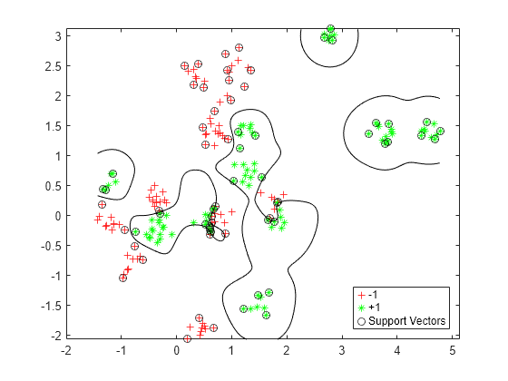
可视化经过优化的分类器。
d = 0.02;
[x1Grid,x2Grid] = meshgrid(min(cdata(:,1)):d:max(cdata(:,1)), ...
    min(cdata(:,2)):d:max(cdata(:,2)));
xGrid = [x1Grid(:),x2Grid(:)];
[~,scores] = predict(Mdl,xGrid);

figure
h(1:2) = gscatter(cdata(:,1),cdata(:,2),grp,'rg','+*');
hold on
h(3) = plot(cdata(Mdl.IsSupportVector,1), ...
    cdata(Mdl.IsSupportVector,2),'ko');
contour(x1Grid,x2Grid,reshape(scores(:,2),size(x1Grid)),[0 0],'k');
legend(h,{'-1','+1','Support Vectors'},'Location','Southeast');
基于新数据计算准确度
生成并分类新的测试数据点。
grnobj = gmdistribution(grnpop,.2*eye(2));
redobj = gmdistribution(redpop,.2*eye(2));

newData = random(grnobj,10);
newData = [newData;random(redobj,10)];
grpData = ones(20,1); % green = 1
grpData(11:20) = -1; % red = -1

v = predict(Mdl,newData);
基于测试数据集计算误分类率。
L_Test = loss(Mdl,newData,grpData)
L_Test =
0.2000
确定哪些新数据点是分类正确的。将正确分类的点格式化为红色方块,将不正确分类的点格式化为黑色方块。
h(4:5) = gscatter(newData(:,1),newData(:,2),v,'mc','**');

mydiff = (v == grpData); % Classified correctly

for ii = mydiff % Plot red squares around correct pts
    h(6) = plot(newData(ii,1),newData(ii,2),'rs','MarkerSize',12);
end

for ii = not(mydiff) % Plot black squares around incorrect pts
    h(7) = plot(newData(ii,1),newData(ii,2),'ks','MarkerSize',12);
end
legend(h,{'-1 (training)','+1 (training)','Support Vectors', ...
    '-1 (classified)','+1 (classified)', ...
    'Correctly Classified','Misclassified'}, ...
    'Location','Southeast');
hold off
