Time Series Anomaly Detection for Cyber Physical Systems in Secure Water Treatment
This example demonstrates how to perform time‑series anomaly detection on the secure water treatment system. The overall goal is to identify abnormal system behavior by learning normal operational patterns from high‑frequency high-dimensional sensor data and detecting deviations that may indicate attacks or system faults. The workflow involves preprocessing the high-frequency sensor data, training a deep learning model on normal operational patterns, evaluating and analyzing its ability to detect various attack scenarios.
Cyber‑Physical Systems (CPSs) integrate computational algorithms with physical components to perform mission‑critical tasks. Due to their large scale and geographic distribution, CPSs rely heavily on networked communication for remote monitoring and control. Anomaly detection in CPSs serves as a critical defensive mechanism by identifying system behaviors that deviate from expected normal operating conditions. These deviations can arise from cyber attacks, where adversaries manipulate control signals or sensor data via communication networks, or from physical attacks that directly affect hardware components such as pumps, valves, or motors. Effective anomaly detection enables early identification of malicious activities, supports preventative maintenance strategies, and facilitates rapid system diagnostics and recovery in industrial control systems.
The Secure Water Treatment System
The Secure Water Treatment (SWaT) dataset [1] is collected from a fully operational water treatment testbed designed specifically to study cyber‑physical security threats. This testbed represents a scaled‑down yet high‑fidelity replica of a modern water treatment facility, implementing a complete six‑stage treatment process that processes approximately 19 liters of water per minute.
To run this example, first go to iTrust Labs and download the dataset. The raw measurement data are organized within the SWAT folder hierarchy. Navigate to the subfolder SWAT\SWaT.A1 & A2_Dec 2015\Physical. The dataset contains two primary files: SWaT_Dataset_Normal_v1.xlsx, which includes sensor and actuator measurements collected during normal system operation, and SWaT_Dataset_Attack_v0.xlsx, which contains measurements recorded during various attack scenarios along with corresponding attack labels. Save those two files in the same directory as the live script.
normalDataFile = fullfile(pwd, "SWaT_Dataset_Normal_v1.xlsx");
attackDataFile = fullfile(pwd, "SWaT_Dataset_Attack_v0.xlsx");
opts = detectImportOptions(normalDataFile,"VariableNamingRule","preserve");
opts = setvartype(opts,'Timestamp','datetime');
opts = setvaropts(opts,'Timestamp','InputFormat','dd/MM/yyyy h:mm:ss a');
normalRaw = readtable(normalDataFile,opts);
attackRaw = readtable(attackDataFile,opts);
The dataset captures real‑world multivariate time‑series measurements obtained from 51 sensors and actuators distributed throughout the plant [1]. These instruments continuously monitor and control various physical and chemical processes, including water levels, flow rates, pressures, pH values, and conductivity. Data are sampled at a frequency of 1 Hz, providing fine‑grained temporal resolution suitable for capturing both gradual process changes and abrupt anomalous events. The complete dataset spans 15 days of operation, consisting of 11 days of normal system operation containing approximately 495,000 observations, followed by 4 days of operation under various attack scenarios comprising approximately 449,919 observations.
The normal operation data contains only benign system behavior, allowing models to learn the typical operational patterns, correlations, and dynamics without contamination from anomalous samples. The attack data, which includes 36 distinct attack scenarios targeting different components and processes, provides a comprehensive evaluation benchmark for assessing detection performance across diverse threat types and severities.
head(normalRaw, 3)
          Timestamp          FIT101    LIT101    MV101    P101    P102    AIT201    AIT202    AIT203    FIT201    MV201    P201    P202    P203    P204    P205    P206    DPIT301      FIT301      LIT301    MV301    MV302    MV303    MV304    P301    P302    AIT401    AIT402    FIT401    LIT401    P401    P402    P403    P404    UV401    AIT501    AIT502    AIT503    AIT504     FIT501       FIT502      FIT503      FIT504    P501    P502    PIT501    PIT502    PIT503     FIT601      P601    P602    P603    Normal/Attack
    _____________________    ______    ______    _____    ____    ____    ______    ______    ______    ______    _____    ____    ____    ____    ____    ____    ____    _______    __________    ______    _____    _____    _____    _____    ____    ____    ______    ______    ______    ______    ____    ____    ____    ____    _____    ______    ______    ______    ______    _________    ________    _________    ______    ____    ____    ______    ______    ______    _________    ____    ____    ____    _____________

    22/12/2015 4:30:00 PM      0       124.31      1       1       1      251.92    8.3134    312.79      0         1       1       1       1       1       1       1       2.561     0.00025622    138.51      1        1        1        1       1       1        0       169.24      0       133.85     1       1       1       1        1      7.4464    175.42    260.7     123.31    0.0015381    0.001409    0.0016644      0        1       1      9.1002      0       3.3485    0.0002563     1       1       1       {'Normal'}
    22/12/2015 4:30:01 PM      0       124.39      1       1       1      251.92    8.3134    312.79      0         1       1       1       1       1       1       1       2.561     0.00025622    138.75      1        1        1        1       1       1        0       169.24      0          134     1       1       1       1        1      7.4464    175.42    260.7     123.31    0.0015381    0.001409    0.0016644      0        1       1      9.1002      0       3.3485    0.0002563     1       1       1       {'Normal'}
    22/12/2015 4:30:02 PM      0       124.47      1       1       1      251.92    8.3134    312.79      0         1       1       1       1       1       1       1       2.561     0.00025622    138.63      1        1        1        1       1       1        0       169.24      0          134     1       1       1       1        1      7.4464    175.42    260.7     123.31    0.0015381    0.001409    0.0016644      0        1       1      9.1002      0       3.3485    0.0002563     1       1       1       {'Normal'}
Explore and Preprocess Data
Understand Normal Operational Behavior
Examine representative sensor measurements from the training data to understand the characteristics of normal system operation. The sensor LIT101 measures the raw water tank level at Stage 1, which is controlled by the motorized valve MV101. This visualization helps us identify the typical temporal patterns in the data, and it reveals any startup transients or initialization periods that should be excluded from model training.
figure()
plot(normalRaw{1:80000, 'Timestamp'}, normalize(normalRaw{1:80000, 'LIT101'}, 'range'), '-b', 'LineWidth', 1.5);
ylabel('LIT101');
xlabel("Time");
title('Normal Behavior in Training dataset')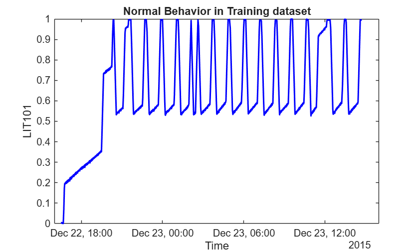
The plot shows that the data collection process began from an empty tank state, and it took approximately 5 hours for the SWaT system to stabilize into its normal operating regime. This startup period exhibits atypical dynamics that do not represent steady‑state operation. Given the 1 Hz sampling rate, this corresponds to approximately 18,000 samples that should be removed before training to ensure the model learns only stable operational patterns.
After the system stabilizes, the LIT101 signal exhibits clear repetitive and cyclic behavior over time. This pattern arises from the integrating nature of tank dynamics combined with threshold‑based control logic: the tank fills until reaching an upper threshold, then empties to a lower threshold, creating regular oscillations. This cyclic behavior is characteristic of many process variables in the SWaT system and suggests that forecasting‑based anomaly detection methods may be particularly effective, as they can learn these predictable patterns and identify deviations from expected trajectories.
Understand Cyber Attacks in Water Treatment
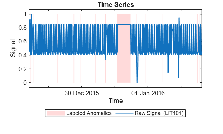
Visualize the attack data to understand what types of anomalies the model will need to detect. The SWaT attack dataset contains 36 distinct attack scenarios with varying characteristics in terms of target location, attack mechanism, duration, and severity. These attacks span multiple categories including single‑stage single‑point attacks that target one sensor or actuator in one process stage, single‑stage multi‑point attacks affecting multiple components in the same stage, and more complex multi‑stage attacks that disrupt coordinated processes across different treatment stages. The attacks range from brief disruptions lasting only a few minutes to prolonged campaigns spanning several hours. Specifically, the shortest recorded attack lasts 101 seconds, while the longest extends to 35,900 seconds (nearly 10 hours). This wide range presents a significant challenge for anomaly detection: the method must be sensitive enough to detect short‑duration attacks with potentially subtle effects, while also maintaining robustness against false alarms during extended normal operations.
testLabels = ~strcmp(string(attackRaw.('Normal/Attack')), "Normal");
testTime = attackRaw.Timestamp;
hPlotSubseqeunce(attackRaw, [], testLabels, "LIT101", testTime)
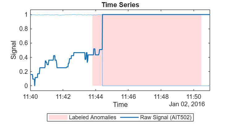
An important consideration when working with the SWaT dataset is understanding how the attack labels correspond to observable changes in sensor data. The provided labels indicate when an attack action was initiated, but this does not always align precisely with when physical anomalies become visible in sensor measurements. This temporal misalignment arises because physical processes have inherent dynamics: after an attack is executed, it takes time for its effects to propagate through the system and manifest as measurable deviations in sensor readings.
Examine a specific attack event between 11:40 and 11:51 on February 1, 2016 to illustrate this phenomenon. The sensor measurements may not show immediate deviation at the labeled attack start time, and conversely, the effects may persist slightly beyond the labeled attack end time. This delay occurs because the labeled intervals are based on when malicious commands were issued, not when the resulting physical changes became detectable in the process state.
This observation has important implications for performance evaluation. Evaluating detection accuracy strictly based on the provided labels may not fully capture the detector's true capability, as it may penalize the model for not detecting attacks during periods when no observable anomaly exists, or reward it for detections that occur slightly outside the labeled interval but align with actual physical deviations.
eventIdx = attackRaw.Timestamp >= datetime('2/1/2016 11:40:00','InputFormat','dd/MM/yyyy HH:mm:ss') & attackRaw.Timestamp <= datetime('2/1/2016 11:51:00','InputFormat','dd/MM/yyyy HH:mm:ss') ;
hPlotSubseqeunce(attackRaw(eventIdx,:), [], testLabels(eventIdx), ["AIT502", "FIT401"], testTime(eventIdx))
Preprocess Data
The raw SWaT dataset contains both sensor measurements and actuator states. For this anomaly detection approach, we make the deliberate choice to train all models using only sensor measurements, explicitly excluding actuator signals from the feature set. This design decision focuses the anomaly detector on identifying deviations in the physical process state rather than changes in control commands.
The rationale for excluding actuators is based on their operational characteristics. Actuator signals in SWaT primarily represent controller intent and frequently change during normal operation as part of routine control actions. Including these signals could introduce spurious anomalies when the controller responds to normal process variations, potentially obscuring physically meaningful deviations. By focusing exclusively on sensor data, the proposed approach targets anomalies that manifest at the process level and are directly observable through changes in the physical state of the system.
The preprocessing pipeline implements several additional steps to ensure data quality. First, based on the earlier signal visualization, the first 18,000 observations are removed from the training data to exclude startup transients and unstable system behavior. Second, features with very low variability (five or fewer unique values) are identified and removed, as these provide minimal information for anomaly detection. After these preprocessing steps, the final feature set consists of 25 sensor signals. The same preprocessing transformations are applied consistently to both training and test data to ensure compatibility.
[trainData, testData] = hPreprocessData(normalRaw, attackRaw);
head(trainData, 3)
    FIT101    LIT101    AIT201    AIT202    AIT203    FIT201    DPIT301    FIT301    LIT301    AIT401    AIT402    FIT401    LIT401    AIT501    AIT502    AIT503    AIT504    FIT501    FIT502    FIT503     FIT504     PIT501    PIT502    PIT503      FIT601
    ______    ______    ______    ______    ______    ______    _______    ______    ______    ______    ______    ______    ______    ______    ______    ______    ______    ______    ______    _______    _______    ______    ______    ______    __________

      0       813.98    261.5     8.4227    423.43      0       2.2088       0       1013.5      0       192.36    1.7007    816.56    7.8642    178.01    273.58    11.958    1.7132    1.2818    0.73873    0.30817    253.78    1.1373    192.9     6.4076e-05
      0       813.91    261.5     8.4227    423.43      0       2.2088       0       1013.5      0       192.36    1.7012    816.41    7.8642    178.11    273.58    11.958    1.7132    1.2819    0.73873    0.30817    253.78    1.1373    192.9     6.4076e-05
      0       814.14    261.5     8.4227    423.43      0       2.2088       0       1013.1      0       192.36    1.7051     816.1    7.8642    178.24    273.58    11.958    1.7132    1.2651    0.73873    0.30817    253.78    1.1373    192.9     6.4076e-05
Train A Deep Time Series DeepAnT Detector
Given the repetitive and cyclic nature of the sensor signals observed during normal operation, a forecasting‑based anomaly detection approach is well‑suited for this problem. The fundamental principle is that if the system is operating normally, future sensor values should be predictable based on recent historical observations. Anomalies can then be identified when actual future observations % deviate significantly from these forecasted values.
For this purpose, DeepAnT is an unsupervised deep learning architecture specifically designed for time‑series anomaly detection. DeepAnT uses a convolutional neural network with a sliding window mechanism to learn normal temporal patterns from historical data. During inference, the model forecasts future values based on a recent observation window, then computes the prediction error between forecasted and actual values. An observation is flagged as anomalous when this error exceeds a predefined threshold.
The configuration of window lengths is critical for balancing detection sensitivity with robustness. The observation window length is set to 1,800 samples, which corresponds to 30 minutes of historical. This duration was selected based on the visualized cycle time of approximately 30 minutes observed in signals like LIT101, ensuring the model can capture complete operational cycles. The detection window length is set to 300 samples (5 minutes), which balances sensitivity to relatively short anomalies while providing sufficient temporal extent to reduce sensitivity to isolated noise % spikes. The network architecture employs 128 convolutional filters, providing adequate model capacity for learning complex multivariate patterns across the 25 sensor channels while maintaining computational efficiency. First filter size is set as 180 to capture long‑term trends and cyclic patterns that span multiple minutes and the second filter size is set as 5 to detect short‑term dynamics and rapid transients. A dropout probability of 0.15 is applied during training to prevent overfitting and improve generalization to unseen data. To accelerate training while maintaining comprehensive coverage, both training and detection strides are set equal to the detection window length (300 samples). Data normalization is applied automatically using range‑based scaling, where minimum and maximum values are computed from the training data and applied consistently to both training and test data to ensure proper scaling.
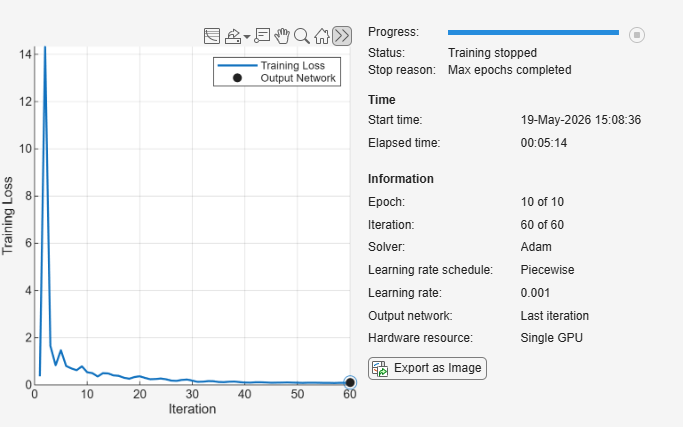
numChannels = size(trainData,2);
detector = deepantAD(numChannels,"ObservationWindowLength", 1800, "DetectionWindowLength",300, "DropoutProbability", 0.15, "NumFilters", 128, ...
    "TrainingStride", 300, "Normalization","range", "FilterSize",[180,5],"DetectionStride",300);
trainingOps = trainingOptions("adam","Plots","training-progress","MaxEpochs",10,"LearnRateSchedule","piecewise","InitialLearnRate",0.001, Verbose=false, MiniBatchSize=256);
trainedDetector=train(detector,trainData{:,:},"TrainingOpts",trainingOps)
trainedDetector =
  DeepantDetector with properties:

    ObservationWindowLength: 1800
      DetectionWindowLength: 300
                 FilterSize: [180 5]
         DropoutProbability: 0.1500
                 NumFilters: [128 128]
             TrainingStride: 300
                  IsTrained: 1
                NumChannels: 25
                     Layers: [13×1 nnet.cnn.layer.Layer]
                      Dlnet: [1×1 dlnetwork]
                  Threshold: 2.4395
            ThresholdMethod: "kSigma"
         ThresholdParameter: 3
          ThresholdFunction: []
              Normalization: "range"
            DetectionStride: 300
After training, apply the detector to the test data to compute anomaly scores for each detection window. Plotting the anomaly scores alongside the automatically learned threshold provides valuable insight into the detector's behavior. The visualization reveals that certain regions of the test data exhibit substantially higher anomaly scores, which likely correspond to attack periods. However, the distribution of anomaly scores suggests that the automatically selected threshold may not optimally separate anomalous subsequences from normal operation. Some regions with elevated scores remain below the automatic threshold, while the threshold might be adjusted to reduce false alarms without sacrificing detection of major anomalies. This observation motivates manual refinement of the threshold.
plot(trainedDetector, testData{:,:}, "PlotType","anomalyScores","MiniBatchSize",256);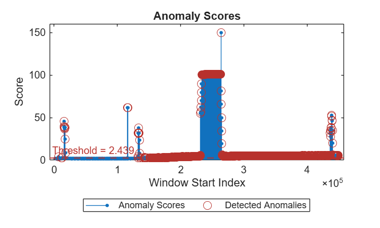
Update Threshold in the Trained Detector
Based on the anomaly score distribution observed in the previous step, we manually update the detector's threshold to improve separation between normal and anomalous behavior.
trainedDetector = updateDetector(trainedDetector,"ThresholdMethod","manual","Threshold",6);
Re‑plotting the anomaly scores with the updated threshold allows us to validate this choice. The updated visualization should show clearer separation, with attack regions more distinctly exceeding the threshold while normal regions remain below it. This threshold tuning process is iterative and can be further refined based on performance metrics computed in subsequent steps.
plot(trainedDetector, testData{:,:}, "PlotType","anomalyScores","MiniBatchSize",256);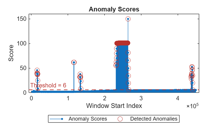
Detect Anomalies in Test Data
The updated detector is evaluated using timeSeriesAnomalyMetrics.In anomaly detection problems, overall classification accuracy is often misleading because the vast majority of samples correspond to normal operation, creating a severe class imbalance. A trivial detector that labels everything as normal could achieve high accuracy while completely failing to identify any attacks. Therefore, precision, recall, and F1 score provide more meaningful assessment of detection capability. Precision measures what fraction of raised alarms correspond to actual attacks, recall measures what fraction of actual attack samples were successfully detected, and the F1 score provides a balanced harmonic mean of these two metrics. Those values show the detection capability of attacks.
YTestPred = detect(trainedDetector, testData{:,:}, "MiniBatchSize",256,"Resolution","sample");
timeSeriesAnomalyMetrics(YTestPred.Labels, testLabels, "Method","point-adjusted")ans=1×7 table
0.9452 2×1 table 2×2 table 0.7605 0.0234 0.8091 0.7174
Visualize the detection results alongside raw sensor measurements and ground truth labels. The visualization reveals an important pattern: much of the reported performance is driven by successful detection of the longest attack sequences, which produce sustained and substantial deviations from normal patterns. These long‑duration attacks generate consistently high anomaly scores, making them relatively easy to detect. However, the visualization also suggests that some shorter attacks may be missed or only partially detected, indicating that detection performance varies significantly with attack duration and magnitude.
hPlotSubseqeunce(testData, YTestPred, testLabels, "AIT502",testTime)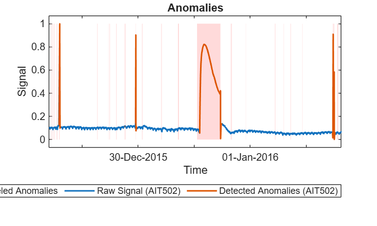
Analyze Subsequence-Level Performance
While sample‑level metrics provide an overall assessment, they do not reveal how effectively the detector identifies individual attack events. A single long attack with high detection recall can dominate the metrics, while numerous short attacks that are completely missed may have minimal impact on the aggregate numbers. To address this limitation, we perform a subsequence‑level analysis that evaluates detection performance for each individual attack event separately.
This analysis treats each contiguous anomalous interval in the ground truth as a distinct subsequence and computes whether it was detected (at least one sample flagged as anomalous), what percentage of its samples were detected, and how long it took to detect after the attack began. This subsequence‑level perspective is often more relevant for operational security, as detecting the presence of an attack quickly is typically more important than detecting every single sample within a long attack sequence.
The results reveal that out of the 36 attack scenarios present in the test data, a subset are successfully detected while others are missed entirely. Examining the characteristics of detected versus missed attacks provides insight into the detector's strengths and limitations. Shorter attacks with smaller perturbations are inherently more difficult to identify because their impact on prediction error may not be sufficiently large to exceed the threshold. The attacks that produce subtle changes in only one or two sensors, or whose effects are quickly compensated by the control system, present particular challenges.
results = hAnalyzeDetection(testLabels, YTestPred.Labels, attackRaw);
=== Detection Analysis Summary ===
Total ground truth subsequences: 35
Subsequences detected (at least 1 prediction): 9

=== Detection Delay (Detected Subsequences Only) ===
Median detection delay: 00:00:00
Max detection delay:    01:02:52
display(results(results.IsDetected == true,1:5))
  9×5 table

    AttackSubsequenceID       StartTimestamp           EndTimestamp        Length    DetectedCount
    ___________________    ____________________    ____________________    ______    _____________

             8             28-Dec-2015 14:16:20    28-Dec-2015 14:28:20      721           721
            14             29-Dec-2015 18:10:43    29-Dec-2015 18:15:01      259             2
            15             29-Dec-2015 18:15:43    29-Dec-2015 18:22:17      395           395
            17             29-Dec-2015 22:55:18    29-Dec-2015 23:03:00      463           463
            22             31-Dec-2015 01:17:08    31-Dec-2015 11:15:27    35900         32128
            31             02-Jan-2016 11:17:02    02-Jan-2016 11:24:50      469           469
            32             02-Jan-2016 11:31:38    02-Jan-2016 11:36:18      281           281
            33             02-Jan-2016 11:43:48    02-Jan-2016 11:50:28      401           401
            34             02-Jan-2016 11:51:42    02-Jan-2016 11:56:38      297           297

	Get insights using Copilot
Investigate the Mismatch Between Labels and Observable Anomalies
A critical insight is that SWaT labels indicate when an attack action was executed at the control level, not when a physical anomaly becomes observable in sensor measurements. Many attacks in the SWaT dataset target actuators or control logic without producing immediate or substantial changes in sensor readings.
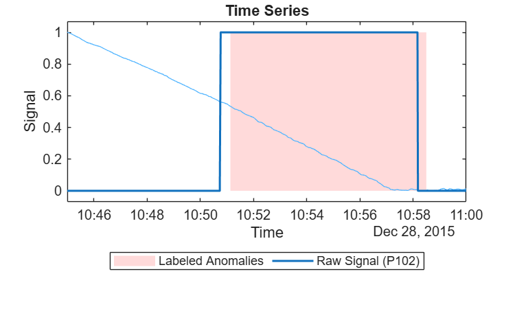
Actuator‑only attacks: Some attacks affect only actuator states without producing measurable changes in physical process variables. Sensor readings remain within normal ranges because the physical process has sufficient buffering capacity or inertia to absorb the disturbance. A concrete example occurs during the attack between 10:45 and 11:00 on December 28, 2015, which targets pump P102.
According to the attack description, this scenario involves manipulating P102 with the intent to cause the pipe between the raw water tank and the second stage to burst. If successful, such a pipe burst would be expected to produce a rapid decrease in the raw water tank level as measured by LIT101. However, examining the actual sensor data reveals no such phenomenon. The LIT101 signal shows only the normal cyclic pattern of gradual water level decrease during the tank draining phase, with no significant change in the rate of level decrease. The absence of observable sensor deviation suggests either that the attack did not achieve its intended physical effect, or that any impact was too subtle to distinguish from normal operational variations. From a purely sensor‑based perspective, this labeled attack interval is indistinguishable from normal operation.
eventIdx = attackRaw.Timestamp >= datetime('28/12/2015 10:45:00','InputFormat','dd/MM/yyyy HH:mm:ss') & attackRaw.Timestamp <= datetime('28/12/2015 11:00:00','InputFormat','dd/MM/yyyy HH:mm:ss') ;
hPlotSubseqeunce(attackRaw(eventIdx,:), [], testLabels(eventIdx), ["P102", "LIT101"], testTime(eventIdx))
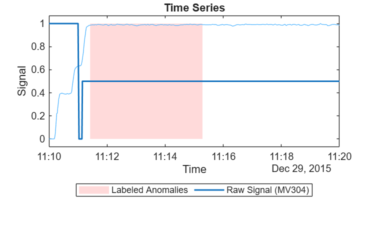
Failed/Delayed Attack: The attack occurring between 11:10 and 11:20 on December 29, 2015 illustrates a failed attack. This attack targets motorized valve MV304, which controls the ultrafiltration drain in Stage 3. The attack attempts to turn off MV304 completely, which would be expected to halt normal operation in Stage 3 and cause observable changes in the differential pressure measured by DPIT301. However, visualization of the actuator state reveals that MV304 does not close to zero as the attack intended. The valve remains partially open, allowing continued operation with minimal disruption. Consequently, the differential pressure sensor DPIT301 shows no significant deviation from its normal operating range. This example demonstrates that not all attack commands successfully alter the physical system state, and failed or incomplete attacks naturally produce no detectable sensor anomalies.
eventIdx = attackRaw.Timestamp >= datetime('29/12/2015 11:10:00','InputFormat','dd/MM/yyyy HH:mm:ss') & attackRaw.Timestamp <= datetime('29/12/2015 11:20:00','InputFormat','dd/MM/yyyy HH:mm:ss') ;
hPlotSubseqeunce(attackRaw(eventIdx,:), [], testLabels(eventIdx), ["MV304", "DPIT301"], testTime(eventIdx))
Helper Functions
function [trainData, testData] = hPreprocessData(trainData, testData)
%hPreprocessData remove actuators columns
dropCols = {'Timestamp', 'Normal/Attack'};
trainData = removevars(trainData, dropCols);
testData = removevars(testData, dropCols);
featureCols = trainData.Properties.VariableNames;
uniqueCounts = varfun(@(c) numel(unique(c)), trainData(:, featureCols), 'OutputFormat', 'uniform');
columnsDropped = featureCols(uniqueCounts <= 5);
trainData(:, columnsDropped) = [];
trainData = trainData(18000:end, :);
testData(:, columnsDropped) = [];
end

function hPlotSubseqeunce(data, pred, labels, featureCol, time)
%hPlotSubseqeunce plot signals with prediction result and ground truth
%labels
if isscalar(featureCol)
y = data.(featureCol);
else
y = data{:,featureCol};
end
y = normalize(y,1, "range");
% Plots
ax = newplot;
ax.NextPlot = 'replace';
fig = ancestor(ax, 'figure');
fig.Position = [100, 100, 500, 300];
anomalyCLI.internal.utils.AnomalyDetection.plotAnomalies(...
    ax, y, featureCol, pred, ...
    1, TrueLabels=labels, Time = time);

set(fig, 'NextPlot', 'replace'); % Will clear listeners if figure's content gets updated.
end


function [results, summary] = hAnalyzeDetection(ground_truth, prediction, data)
% hAnalyzeDetection Analyze detection performance for each ground truth subsequence

% Find start and end indices of each ground-truth subsequence
diff_gt = diff([false; ground_truth; false]);
starts = find(diff_gt == 1);
ends   = find(diff_gt == -1) - 1;

num_subsequences = numel(starts);

% Preallocate arrays
start_timestamps        = NaT(num_subsequences, 1);
end_timestamps          = NaT(num_subsequences, 1);
subsequence_lengths     = zeros(num_subsequences, 1);
detected_counts         = zeros(num_subsequences, 1);
is_detected             = false(num_subsequences, 1);

% New: detection delay fields
first_detection_index     = NaN(num_subsequences, 1);
first_detection_timestamp = NaT(num_subsequences, 1);
detection_delay           = duration(NaN, NaN, NaN); % NaN duration

% Analyze each subsequence
for i = 1:num_subsequences
    start_idx = starts(i);
    end_idx   = ends(i);

    % Extract timestamps
    start_timestamps(i) = data.Timestamp(start_idx);
    end_timestamps(i)   = data.Timestamp(end_idx);

    % Subsequence length
    subsequence_lengths(i) = end_idx - start_idx + 1;

    % Count detections inside this subsequence
    pred_seg = prediction(start_idx:end_idx);
    detected_counts(i) = sum(pred_seg);

    % Detected?
    is_detected(i) = detected_counts(i) > 0;

    % First detection time and delay
    if is_detected(i)
        rel_idx = find(pred_seg, 1, 'first');              % first 1 within segment
        first_idx = start_idx + rel_idx - 1;              % absolute index
        first_detection_index(i) = first_idx;
        first_detection_timestamp(i) = data.Timestamp(first_idx);

        % Detection delay as duration (works with datetime)
        detection_delay(i) = first_detection_timestamp(i) - start_timestamps(i);
    else
        detection_delay(i) = duration(NaN, NaN, NaN);
    end
end

results = table((1:num_subsequences)', ...
    start_timestamps, ...
    end_timestamps, ...
    subsequence_lengths, ...
    detected_counts, ...
    is_detected, ...
    'VariableNames', { ...
    'AttackSubsequenceID', ...
    'StartTimestamp', ...
    'EndTimestamp', ...
    'Length', ...
    'DetectedCount', ...
    'IsDetected'});

% Summary statistics
summary.total_subsequences = num_subsequences;
summary.detected_subsequences = sum(is_detected);

% New: delay stats (only for detected)
detected_delays = detection_delay(is_detected);
summary.median_detection_delay = median(detected_delays, 'omitnan');
summary.max_detection_delay    = max(detected_delays);

% Display summary
fprintf('\n=== Detection Analysis Summary ===\n');
fprintf('Total ground truth subsequences: %d\n', summary.total_subsequences);
fprintf('Subsequences detected (at least 1 prediction): %d\n', summary.detected_subsequences);

fprintf('\n=== Detection Delay (Detected Subsequences Only) ===\n');
fprintf('Median detection delay: %s\n', string(summary.median_detection_delay));
fprintf('Max detection delay:    %s\n\n', string(summary.max_detection_delay));
end
References
[1] A. P. Mathur and N. O. Tippenhauer, "SWaT: a water treatment testbed for research and training on ICS security," 2016 International Workshop on Cyber-physical Systems for Smart Water Networks (CySWater), Vienna, Austria, 2016, pp. 31-36, doi: 10.1109/CySWater.2016.7469060.
Copyright 2026 The MathWorks, Inc.