Dynamic Selection of Optimal High PRF Sets for Airborne Radar

Introduction to Waveform Design

Waveform optimization aims to determine the waveform or often the set of waveforms that can meet multiple key performance indicators (KPIs). These waveforms must achieve this while contending with the hardware limitations of the platform. Analysis and visualization tools in Radar Toolbox™, including Radar Designer and blind zone-related functions (e.g., blindrangemap, blindvelocitymap, and blindzonemap), facilitate waveform design and optimization. This example shows how you can determine a set of pulse repetition frequencies (PRFs) that maximize the range of the first blind zone while maintaining a high probability of detection (Pd) for a variety of target sizes and fluctuation models. Blind ranges, Doppler velocity, range migration, and probability of detection were considered and their interdependence is visualized. The platform under consideration is a monostatic, X-band (8-12 GHz), airborne pulsed radar, and this example focuses solely on the high PRF (HPRF) regime. Medium and low PRF waveforms can also be used on such a platform and can be configured using a similar process.

Why Not Just Use a Single Waveform?

A single waveform, by itself, typically cannot meet all of the necessary KPIs. For example, if you are only seeking to maximize the Pd outside of a blind zone, you may be tempted to choose a single PRF and transmit many pulses over a long dwell time. This creates frequent blind zones which lowers the Pd at regular intervals, as demonstrated in the Multiple CPIs of the Same Waveform section. Conversely, combining a diverse and intentional set of waveforms, or staggering PRFs, can greatly reduce such blind zones. To realize the potential benefits of using different waveforms, the waveform designer must consider how the ambiguities and shortcomings in each waveform can be mitigated with the other waveforms.

PRF Regimes

Waveforms can broadly be divided into 3 PRF regimes:

High PRF (HPRF):

Medium PRF (MPRF):

Low PRF (LPRF):

Hardware Constraints for All Waveforms

Hardware limitations vary by platform and must be considered for all waveforms. Below, a few hardware constraints are listed that are respected throughout this example.

bandwidth = 50e6; % (Hz)
c = physconst('lightspeed');
rangeRes = bw2rangeres(bandwidth,c) % (m)

rangeRes = 
2.9979

fc = 10e9; % (Hz) X-band radar
lambda = freq2wavelen(fc);

Maximum Unambiguous Range and Eclipsing

Radars are able to determine the range of targets by transmitting pulses and then measuring the times of flight of the reflections generated by those targets. In most cases, radars transmit these pulses at regular pulse repetition frequencies or PRFs. Ambiguity in a target's range measurement is introduced when a target is so far that the reflected pulse is only received after the next pulse is transmitted. This phenomenon can lead to uncertainty in which transmission the reflected pulse originated from. The maximum range without this ambiguity, i.e. the farthest a target can be while its reflection still arrives before the next transmission, is known as the maximum unambiguous range. Lower PRFs allow more time for the reflected signals which explains why maximum unambiguous range is inversely proportional to PRF.

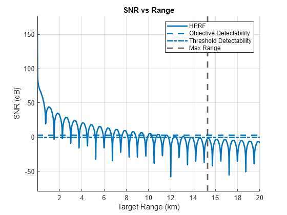
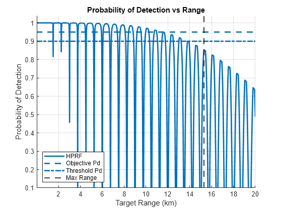
In addition to ambiguous range measurements, the repeated transmission of pulses leads to the issue of eclipsing in some radar systems. Eclipsing refers to the phenomenon where the radar receiver is unable to detect returned signals because the radar transmitter is active. This typically occurs when the transmitted pulse is long enough that the receiver is effectively "blinded" or "eclipsed" by the transmission, preventing it from detecting reflections that return during this period. Because this occurs every time the radar is transmitting, these blind ranges occur at multiples of the maximum unambiguous range. More information on the impact of eclipsing in pulsed radars can be found in Introduction to Scanning and Processing Losses in Pulse Radar and Modeling Radar Detectability Factors. For HPRF signals, negative impacts of eclipsing are quite pervasive because pulses are transmitted so frequently. In the figures below, you can see the impact of eclipsing for a PRF of 200kHz, an operating frequency of 10 GHz and a pulse width of 1 microsecond. The steep drops in SNR and probability of detection are where eclipsing occurs.

% The following plots are generated by the Radar Designer app 
% and can be exported by clicking "Export Detectability Analysis Script" 
% in the export menu in the app toolstrip
run("eclipsing_example.m")

Maximum Unambiguous Doppler

HPRF waveforms are designed to allow for the measurement of high Doppler velocities without ambiguity, which is critical for accurately tracking fast-moving targets. For this example, consider a radar platform that can travel up to Mach 1 and targets that can travel up to Mach 2. This scenario can lead to targets that have a relative velocity of up to Mach 3 or 1,029 m/s. The maximum unambiguous velocity, ${\mathit{v}}_{\mathit{u}}$, can be expressed as

${\mathit{v}}_{\mathit{u}}=\frac{\lambda \cdot \mathrm{PRF}}{4}>1029\frac{\mathit{m}}{\mathit{s}}$.

Solving for $\mathrm{PRF}$ and substituting the one-way Doppler shift, $\frac{{\mathit{v}}_{\mathit{u}}}{\lambda }$, with speed2dop, the PRF can be computed as follows:

vu = 1029; % (m/s)
minPRF = 4*speed2dop(vu,lambda) % (Hz)

minPRF = 
1.3729e+05

Addressing Blind Ranges and Co-Ambiguous Ranges

As mentioned above, eclipsing causes blind zones in the range dimension where detection is difficult or even impossible. When designing a set of waveforms, one must pay close attention to how these blind zones overlap. Ideally, the only overlaps are beyond the ranges under consideration. In order to achieve this, one should pick PRFs that are coprime with one another. This results in a set of waveforms where each waveform has a coprime number of equally sized range bins compared to the other waveforms. This is useful because the least common multiple of coprime numbers is their product, i.e. perfect overlap of the blind zones is maximized in range.

In addition to being coprime, the sizes of the blind zones must also be accounted for. If the blind zones take up multiple range bins (which is often the case), then blind zones can partially overlap at ranges closer than a complete overlap between waveforms. Below are three plots that display these phenomena with a pulse width of 1 microsecond and the first PRF around 200 kHz.

pulsewidth = 1e-6; % (s) Duration of the transmitted pulse

subplot(131)
helperPlotBlindRanges([200 164]*1e3, pulsewidth, 10e3) % Not coprime
subplot(132)
helperPlotBlindRanges([199 197]*1e3, pulsewidth, 10e3) % Coprime but PRFs are too close
xlabel(['Black Regions are' newline 'Blind Zones' newline '(PRFs are too close)'])
subplot(133)
helperPlotBlindRanges([199 166]*1e3, pulsewidth, 10e3) % Coprime and PRFs are far enough apart

On the right, you can see that selecting waveforms with coprime PRFs of 199 and 164 kHz results in the first blind zone at around 4.5 km, whereas choosing a similar non-coprime PRF combination of 200 and 164 kHz results in the first blind zone at 3.8 km and a second blind zone at 4.6 km. The blind zones are widest where there is complete overlap. PRFs at 199 and 197 kHz are spaced too close together and result in blind zones at much closer ranges due to partial overlapping, despite being coprime.

Optimize PRF Spacing for Multiple Waveforms

One may want to design the second PRF so that the first partial overlap is at the farthest range possible. To determine the second PRF analytically, use the following steps:

% Compute the maximum range
firstPRF = 199e3;
firstPRI = 1/firstPRF;
maxRange = time2range(firstPRI,c);
blindLength = time2range(pulsewidth,c);
rangeToClear = maxRange + blindLength;
newPRI = range2time(rangeToClear,c);
newPRF = 1/newPRI % (Hz)

newPRF = 
1.6597e+05

This method can be time consuming and cumbersome when considering more than two waveforms. Use the Radar Toolbox™ blindrangemap function to display the blind zones and quickly choose PRFs that would complement each other. Use the code below and look closely at the region in the plot at 0.8 km. Notice whether the blind zone from the waveform PRF on the right overlaps with the blind zone on the left. To maximize the effectiveness of the second waveform, set the second PRF so that the first bling zone narrowly avoids any overlap. Consistent with the analytical approach above, this occurs when the second PRF is set 166 kHz.

R = linspace(0,5e3,1000); % (m) ranges of interest
prf2 = 166; % (kHz)
blindrangemap(R,[199,prf2]*1e3,blindLength)

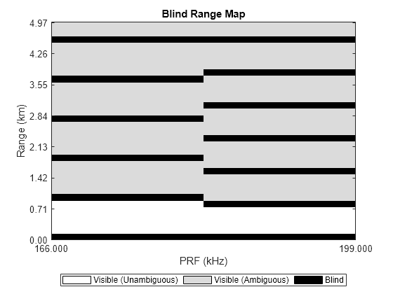
Moreover, this graphical tool can make it easier to choose a third PRF that further extends the range where all three waveforms' blind zones first overlap. Notice that the first three blind zones (after the initial transmission at 0 meters) all just miss each other around 0.8 km and do not overlap.

HPRFs = [199,166,141]*1e3; % (kHz)
blindrangemap(R,HPRFs,blindLength)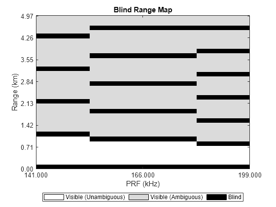

helperPlotBlindRanges(HPRFs, pulsewidth, 20e3)

Adding the third PRF extends the range without any blind zones to over 18 km. It was under 5 km with just two waveforms.

Ambiguity in Range and Velocity

Only blind ranges are considered in this example using blindrangemap. Radar Toolbox™ also includes blindvelocitymap for blind velocities and blindzonemap which considers blind zones in both range and velocity simultaneously to get a unified picture of all the blind zones for the range-Doppler response.

Doppler Resolution and Range Migration

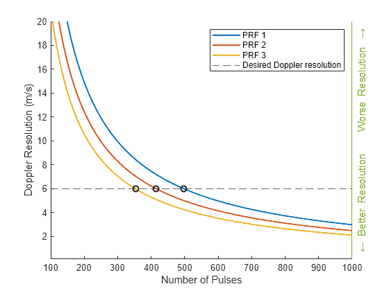
Doppler resolution in meters per second can be computed with the following equation ${\mathit{v}}_{\mathrm{res}}=\frac{\lambda \cdot \mathrm{PRF}}{2\mathit{N}}$ where $\mathit{N}$is the number of pulses in a coherent processing interval (CPI). Let's assume you want the Doppler resolution to be 6 m/s. How many pulses are needed for each waveform? You can compute this analytically using the equation immediately above.

At the same time, one must consider the length of the CPI. If you aim to get a Doppler resolution that is too fine, then the CPI may become so long that a fast moving target changes range bins before all CPIs/waveforms have completed. This is called range migration or range walk and can add difficulty to the task of detection. The relationship between the Doppler resolution and the CPI can be seen by substituting $\frac{\mathrm{PRF}}{\mathit{N}}$ with $\frac{1}{{\mathit{T}}_{\mathrm{CPI}}}$ . With that, the above equation becomes ${\mathit{v}}_{\mathrm{res}}=\frac{\lambda }{{2\mathit{T}}_{\mathrm{CPI}}}$.

dopResKPI = 6; % (m/s) The desired Doppler resolution

nPRFs = numel(HPRFs);
% Number of pulses to achieve a certain Doppler resolution
minPulses = lambda*HPRFs/(2*dopResKPI);
CPIs = minPulses./HPRFs * 1e3; % (ms) Same for all waveforms so choosing first element in display statement

helperDopplerResolutionPlot(dopResKPI, minPulses, HPRFs, lambda)

disp(['A Doppler resolution of ' num2str(dopResKPI) ' m/s requires a CPI of ' num2str(CPIs(1)) ' ms.' newline] )

A Doppler resolution of 6 m/s requires a CPI of 2.4983 ms.

for idx = 1:nPRFs
    disp(['PRF: ' num2str(HPRFs(idx)/1e3) ' kHz,     Min # of Pulses: ' num2str(ceil(minPulses(idx)))])
end    

PRF: 199 kHz,     Min # of Pulses: 498
PRF: 166 kHz,     Min # of Pulses: 415
PRF: 141 kHz,     Min # of Pulses: 353

When Does Range Migration Occur?

Let's assume all three waveforms' CPIs are transmitted sequentially such that one dwell is [Waveform1, Waveform2, Waveform3]. Then one can define range migration as the event when a target changes range bins over the duration of one dwell, or all three CPIs. To compute the minimum velocity when range migration occurs, modify the equation for velocity $\mathit{v}=\frac{\Delta \mathit{d}}{\Delta \mathit{t}}$ to get ${\mathit{v}}_{\max }=\frac{{\mathrm{range}}_{\mathrm{res}}}{3*\mathrm{CPI}}$. Thus, for the given range and Doppler resolution, the minimum Doppler velocity when range migration occurs is:

vMigration = rangeRes/sum(CPIs)*1e3 % (m/s)

vMigration = 
400

If this velocity is too low for the application in question, then you can slide the Doppler resolution above to be less precise and watch vMigration increase.

Probability of Detection

Many of the radar parameters also have an impact on the ability for a radar to detect targets. For example, in the discussion about blind zones, you saw how pulse width effects the size of the blind zone and how PRF affects the frequency of the blind zones. These blind zones of course lead to poor detection performance at regular intervals in range. Then you saw how staggering PRFs can help to reduce the prevalence of such blind zones. The subsequent section showed how the number of pulses affects Doppler resolution and range migration. This section addresses blind zones and the number of pulses again and shows their impacts on the probability of detection for a given target. And just as concluded above, the following simulations show that staggered PRFs provide a unique advantage in their ability to improve Pd. For this example, let the desired Pd be .9 or 90%.

You can explore the probability of detection using the Radar Designer app by designing waveforms and plotting the resulting Pd. The app configuration discussed below can be opened with the following command.

radarDesigner('HPRF.mat')

Define the Waveforms

First, input the first waveform into the app. The radar panel should look like the screenshot below. The app also allows you to include more advanced features like non-free space environments as well as other losses and gains that are beyond the scope of this example.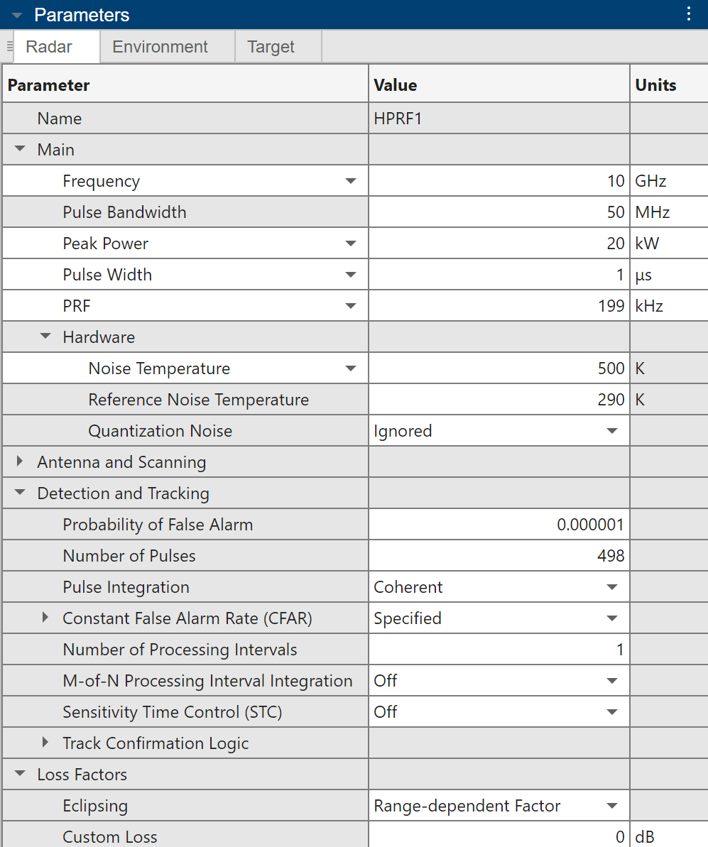

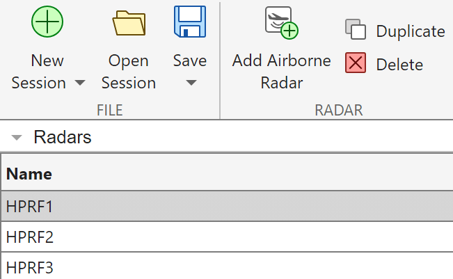
Next, to create the other two waveforms, go to the toolstrip at the top and choose to duplicate this waveform. Once duplicated, rename the additional waveforms, and change their PRF and number of pulses according to the computed values in the previous section.

Define the Target

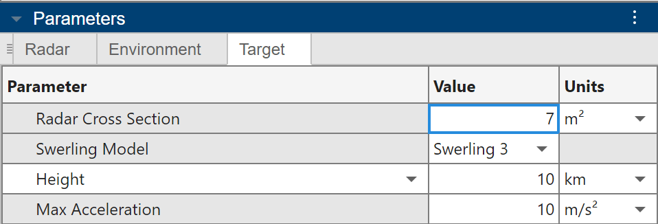
Next, go to the target panel on the left of the Radar Designer app and define the parameters of the target. The Max Acceleration property is only used in the Track Confirmation Logic section in the radar panel which is not used in this example so feel free to leave that as the default value. This target has a 7 ${\mathit{m}}^2$ fluctuating RCS approximated by a Swerling 3 target model. Moreover, the target height is set to 10 km which matches the antenna height of the radar. Equivalent heights and no antenna tilt angle models a scenario where the target is at the center of the main antenna beam.

Maximum Range of Detection of a Single CPI

Navigate to the toolstrip at the at the top and then select the Metric dropdown menu so that it allows you to set a Pd constraint if does not already. Set the constraint to .9 (90%).

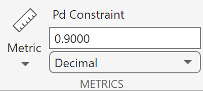
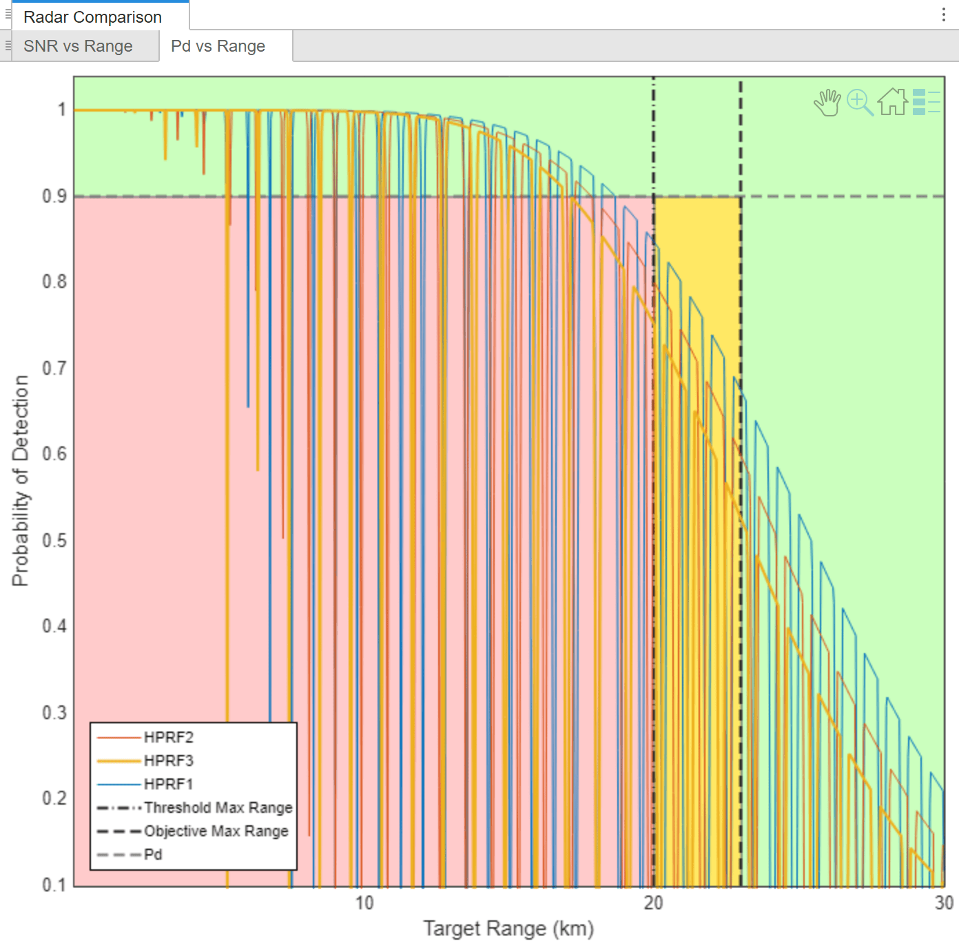
Now look at the metrics table and pay attention to the Max Range. This is the maximum detectable range of the target after 1 CPI for a Pd of 90%. For all ranges greater than the ranges computed in the table, the probability of detection is below 90%. The inverse however is not true. Because of eclipsing, there are ranges less than the maximum range with fading, i.e. ranges with a Pd less than 90%.

The threshold and objective maximum ranges can be set according to your needs as well. Values below the threshold should be values that would not meet critical design requirements. Values above the threshold and below the objective are allowed but fall short of the project goals. Lastly, values above the objective meet or exceed all project expectations.

To see the Pd for every range, navigate to the toolstrip at the top and select Pd vs Range. This option displays the Pd as a function of range for all three waveforms for the specified target. Change the radar, environment, and target properties to see how each impacts the SNR and Pd. The SNR vs Range and the Pd vs range curves can both be exported to a MATLAB script under the Export dropdown menu by clicking the option Export Detectability Analysis MATLAB Script.

Increasing Pd with Multiple CPIs

Increasing the number of CPIs is one way to increase the SNR and Pd. There are multiple ways to increase the number of CPIs. This example discusses three such ways below.

Single PRF

Staggered PRFs (As in the Earlier Sections)

Multiple CPIs with the Same PRF

Navigate to radar panel on the left and change the Number of Processing Intervals for each waveform to 3 to keep things consistent with the number of waveforms in a dwell as described in the earlier section on range migration.

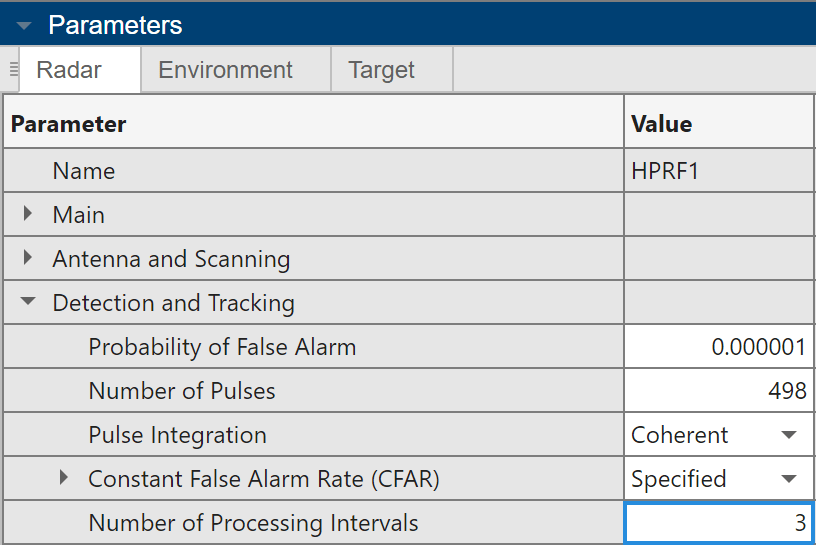
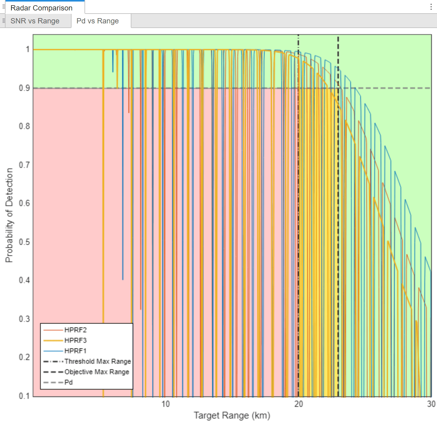
This incoherently integrates the CPIs which already coherently integrated the pulses within the CPI. You can click on Export Detectability Analysis MATLAB Script in the export menu to see precisely how this is implemented. While this does increase the maximum range of each waveform, this does not address the issue of eclipsing since this method uses the same PRF for each repeated CPI. As a result, before the maximum range, there are many ranges for each waveform where the Pd falls well below 90% as seen earlier in this section.

Multiple CPIs of the Same PRF using M-of N Processing Interval Integration

M-of-N processing interval integration searches for targets in each CPI individually and then registers a detection if the same target appears in at least M CPIs out of a total of N CPIs. To enable this, set M-of N Processing Interval Integration to On and set the Number of Processing Intervals with Detection to 1. This means that just one appearance within the three CPIs results in a detection.

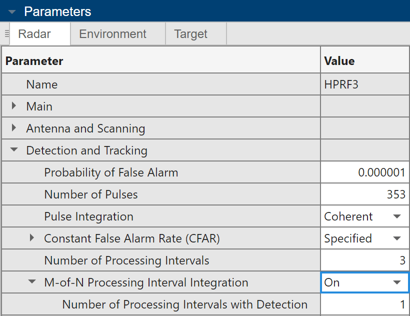
The 1-of-3 decision rule is more aggressive then just increasing the number of CPIs leading to an increase in Pd. However, like the incoherent CPI integration, this still does not address the issue of blind zones at ranges closer than the maximum range as conveyed by the many blind zones in the figure below.

Multiple CPIs of Staggered PRFs using M-of N Processing Interval Integration

As shown in earlier parts of this example, using staggered PRFs can reduce the frequency of blind zones in the range dimension. Using staggered PRFs not only increases the maximum detectable range but also greatly increases the reliability of the detector for the ranges up to the maximum detectable range. Again, consider the 1-of-3 detection rule where just one detection among the three waveforms/CPIs constitutes a detection. Now, to solve for the aggregate Pd using all three waveforms, let $\mathit{P}\left(\mathit{A}\right)$ be the probability that CPI 1 detects a target, $\mathit{P}\left(\mathit{B}\right)$ be the probability that CPI 2 detects a target, and $\mathit{P}\left(\mathit{C}\right)$ be the probability that CPI 3 detects a target. Then, the probability that at least one CPI registers a detection is $1-\mathit{P}\left(\overline{\mathrm{ABC}}\right)$ where the bar represents the compliment of the event occurring. In other words, this is equal to 1 minus the probability that every CPI has a missed detection. For this example, you can assume each CPI is independent giving us the expression $1-\mathit{P}\left(\bar{\mathit{A}}\right)\mathit{P}\left(\bar{\mathit{B}}\right)\mathit{P}\left(\bar{\mathit{C}}\right)$. Lastly, this can be further changed to

$1-\left(1-\mathit{P}\left(\mathit{A}\right)\right)\left(1-\mathit{P}\left(\mathit{B}\right)\right)\left(1-\mathit{P}\left(\mathit{C}\right)\right)$.

The final equation above shows that one can compute the 1-of-3 Pd for the three different waveforms using the individual Pd of each waveform. To compute this for each waveform over all ranges, go to the Export dropdown menu and click the option Export Detectability Analysis MATLAB Script. For your convenience, this example uses already exported scripts with the unnecessary plots commented out.

[HPRF1_pd,ranges] = helperRunAnalysis("HPRF1.m");
HPRF2_pd          = helperRunAnalysis("HPRF2.m");
HPRF3_pd          = helperRunAnalysis("HPRF3.m");
staggeredPd = helperTotalPd([HPRF1_pd HPRF2_pd HPRF3_pd]); % The equation above

figure('Name','Pd vs Range');
hAxes = gca;
radarmetricplot(ranges*1e-3,staggeredPd,.9, ...
    'MaxRangeRequirement',[23 20], ...
    'RadarName',{'Staggered PRF Radar'}, ...
    'MetricName','Probability of Detection', ...
    'RequirementName','Pd', ...
    'RangeUnit','km', ...
    'ShowStoplight',true, ...
    'Parent',hAxes);
ylim(hAxes,[0.1 1.04]);
legend('Location','southwest')

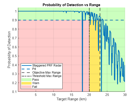
maxRange = helperComputeMaxRange(staggeredPd,ranges,.9) % (km)

maxRange = 
23.9039

The above plot shows how staggering the PRFs impacts the Pd by reducing the amount of blind zones. While the maximum range of 1-of-3 integration using only PRF1 does lead to a higher maximum range (due to longer aggregate time of transmission), using staggered PRFs greatly reduces areas with drops in Pd due to eclipsing.

Summary

This example showed how Radar Toolbox™ can make the process of waveform design much more intuitive with its analytical and visual tools. Blind ranges, Doppler velocity, range migration, and probability of detection were considered and their interdependence was visualized. Lastly, this example clearly demonstrated some of the benefits of staggered PRFs and how Radar Toolbox™ can make designing such sets of waveforms much simpler.

References

Helper Functions

% Plots the intersections of the blind zones when multiple PRFs are used
function helperPlotBlindRanges(prfs,pulsewidth,maxRange)
    validateattributes(prfs,{'double'},{'>',1000}) % make sure the input PRFs are greater than 1 kHz
    nPRF = numel(prfs);
    iscp = iscoprime(prfs/1e3);
    Rmin = time2range(pulsewidth); % (m) blind zone length
    R = linspace(0,maxRange,1000);
    
    BRM = blindrangemap(R,prfs,Rmin);
    BRMComposite = nPRF - sum(BRM,2) > 0;
    
    imagesc(1,R/1e3,BRMComposite)
    colormap("gray")
    set(gca,'XTick',[])
    set(gca,'YDir','normal')
    ylabel('Range (km)')
    xlabel(['Black Regions are' newline 'Blind Zones'])
    if iscp
        title(['PRFs [' num2str(prfs/1e3) '] kHz' newline 'are Coprime'])
    else
        title(['PRFs [' num2str(prfs/1e3) '] kHz' newline 'are NOT Coprime'])
    end
end

% Plotting function for the Doppler resolution vs the number of pulses
function helperDopplerResolutionPlot(dopResKPI, minPulses, HPRFs, lambda)
    figure
    hold on
    worstDopRes = 20; % (m/s)
    nPulses = 100:1000; % Search space of number of pulses
    
    dopRes = lambda * HPRFs ./ (2 * nPulses');
    lines = plot(nPulses,  dopRes, 'LineWidth',1.5);
    set(lines,{'DisplayName'},{'PRF 1';'PRF 2';'PRF 3'})
    scatter(ceil(minPulses),dopResKPI*ones(3,1),'HandleVisibility','off','LineWidth',1.5)
    yline(dopResKPI,'--','DisplayName','Desired Doppler resolution')
    ylim([0.1 worstDopRes])
    xlabel('Number of Pulses')
    ylabel('Doppler Resolution (m/s)')
    yyaxis right
    ylabel('\leftarrow Better Resolution    Worse Resolution \rightarrow')
    yticks([])
    legend
end

% The equation for 1-of-3 integration Pd
function totalPd = helperTotalPd(Pds)
    totalPd = 1-prod(1-Pds,2);
end

% Runs the exported analysis file and outputs Pd and range vectors
function [availablePd, ranges] = helperRunAnalysis(analysisScript)
    run(analysisScript)
    ranges = target.ranges;
end

% Computes the max range of a Pd curve
function maxRange = helperComputeMaxRange(PdCurve,ranges,requiredPd)
    idx = find(PdCurve > requiredPd, 1,'last');
    maxRange = ranges(idx)/1e3;
end

References

Melvin, William L., Scheer, Jim. Principles of Modern Radar: Radar applications. Volume III. United States: SciTech Publishing, 2014.