Improving Weather Radar Moment Estimation with Convolutional Neural Networks
This example shows how to train and evaluate convolutional neural networks (CNN) to improve weather radar moment estimation. First, it shows how to use the weatherTimeSeries function in the Radar Toolbox™ to simulate time series data from the Next Generation Weather Radar (NEXRAD) Level-II data. More information about the NEXRAD data and their physical meaning can be found in the Simulating a Polarimetric Radar Return for Weather Observation example. Then, the simulated time series data is processed by the traditional Pulse-Pair-Processing (PPP) method for radar moment estimation. The estimates are compared with NEXRAD Level-II truth data, from which root mean squared error (RMSE) is obtained for each radar moment. Finally, a convolutional neural network from the Deep Learning Toolbox™ is used to improve the estimation accuracy, which is shown to achieve lower RMSE than PPP method.
Radar System Parameters
The NEXRAD radar system parameters are specified as follows. It is assumed to operate at a frequency of 3 GHz and a pulse repetition frequency (PRF) of 1200 Hz with a radar constant of 80 dB.
fc = 3e9;
lambda = freq2wavelen(fc);
prf = 1200;
radarConst = 80;
rng('default');
Prepare the Data
In this example, 50 datasets collected by NEXRAD are employed, where 45 datasets are used for training and 5 datasets are used for testing. Each dataset has 4 dimensions, where the first dimension is azimuth, the second dimension is range, the third dimension is weather radar moment, and the fourth dimension is image. Each image covers an area of 0 degrees to 45 degrees in azimuth and 5 km to 45 km in range with a range resolution of 250 m.
azimuth = 0:45;
range = (5:0.25:45)*1e3;
Nazimuth = numel(azimuth);
Ngates = numel(range);
Nmoments = 6;
Npulses = 64;
Nimages = 50;
imgs = zeros(Nazimuth,Ngates,Nmoments,Nimages);
trainSet = 1:45;
testSet = 46:50;
Download the dataset which include NEXRAD Level-II data and pretrained networks, and unzip the data into the current working directory.
dataURL = 'https://ssd.mathworks.com/supportfiles/radar/data/NEXRAD_Data.zip';
unzip(dataURL);
Load the NEXRAD Level-II data into workspace.
filename = 'NEXRAD_Data.mat';
load(filename,'resps');
Time Series Data Simulation and Radar Moment Estimation
The weatherTimeSeries function in the Radar Toolbox™ is used to simulate time series data from the NEXRAD Level-II data as ground truth. Then pulse pair processing method is applied to the simulated time series to estimate the radar moment data, which is composed of reflectivity (ZH), radial velocity (Vr), spectrum width (SW), differential reflectivity (ZDR), correlation coefficient (Rhohv), and differential phase (Phidp). Then, the estimates are compared with NEXRAD ground truth, from which the root mean squared error (RMSE) is averaged over the entire test dataset. As a reference, the data quality specifications of NEXRAD are also listed.
for ind = 1:Nimages
    for ii = 1:Nazimuth
        Pr = resps(ii,:,1,ind)-radarConst-mag2db(range/1e3);
        Vr = resps(ii,:,2,ind);
        SW = resps(ii,:,3,ind);
        ZDR = resps(ii,:,4,ind);
        Rhohv = resps(ii,:,5,ind);
        Phidp = resps(ii,:,6,ind);
        [Vh,Vv] = weatherTimeSeries(fc,Pr,Vr,SW,ZDR,Rhohv,Phidp,...
            'PRF',prf,'NumPulses',Npulses);
        moment = helperPulsePairProcessing(Vh,Vv,lambda,prf);
        imgs(ii,:,1,ind) = moment.Pr+mag2db(range.'/1e3)+radarConst;
        imgs(ii,:,2,ind) = moment.Vr;
        imgs(ii,:,3,ind) = moment.SW;
        imgs(ii,:,4,ind) = moment.ZDR;
        imgs(ii,:,5,ind) = moment.Rhohv;
        imgs(ii,:,6,ind) = moment.Phidp;
    end
end
helperErrorStatistics(imgs(:,:,:,testSet),resps(:,:,:,testSet));
    MomentName    RMSE_Avg    Specification       Unit
    __________    ________    _____________    __________

    {'ZH'   }       1.89             1         {'dB'    }
    {'Vr'   }       0.53             1         {'m/s'   }
    {'SW'   }       0.67             1         {'m/s'   }
    {'ZDR'  }       0.44           0.2         {'dB'    }
    {'Rhohv'}      0.013          0.01         {'N/A'   }
    {'Phidp'}       3.12             2         {'degree'}
As shown in the table above, due to sampling and estimation error, the RMSE of PPP estimates for ZH, ZDR, Rhohv, and Phidp of the test dataset doesn't always meet NEXRAD data quality specifications. NEXRAD ground truth images of the first case in the test dataset are plotted below. In addition, the radar images of PPP estimates minus ground truth are also plotted, where the noisy area indicates larger estimation errors.
helperImagePlot(range,azimuth,resps(:,:,:,testSet(1)),'NEXRAD Ground Truth',0);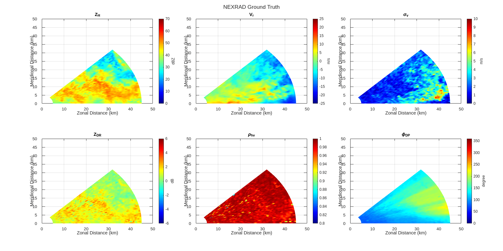
helperImagePlot(range,azimuth,imgs(:,:,:,testSet(1))-resps(:,:,:,testSet(1)),'PPP Estimates minus Ground Truth',1);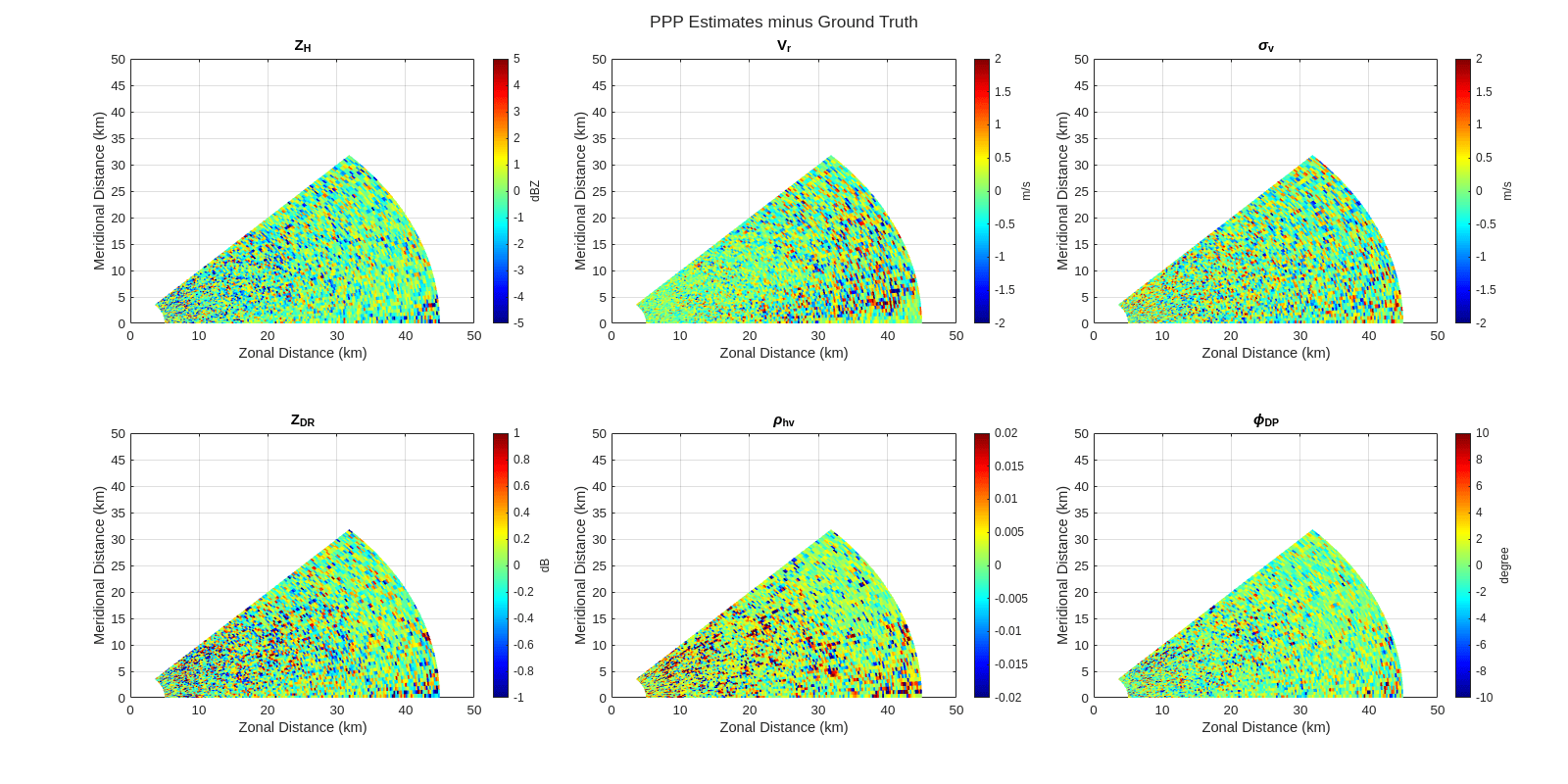
To better visualize the distribution of estimation errors, the histogram of PPP estimates minus the NEXRAD ground truth of each radar moment is plotted, which shows all the PPP estimates have a wide range of estimation error.
helperHistPlot(imgs(:,:,:,testSet(1)),resps(:,:,:,testSet(1)),'Histogram of PPP Estimates minus Ground Truth');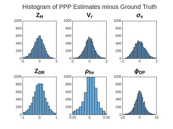
Network Architecture
To improve radar moment estimation accuracy, we design a CNN whose network architecture is shown below.
layers = [
    imageInputLayer([Nazimuth Ngates 1],"Normalization","none");
    convolution2dLayer([8 8],16,"Padding","same")
    reluLayer
    batchNormalizationLayer
    convolution2dLayer([8 8],8,"Padding","same")
    reluLayer
    batchNormalizationLayer
    convolution2dLayer([4 4],1,"Padding","same")];
dlnet = dlnetwork(layers);
figure;
plot(dlnet);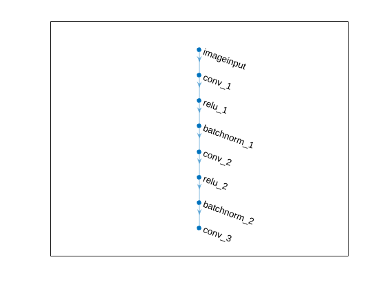
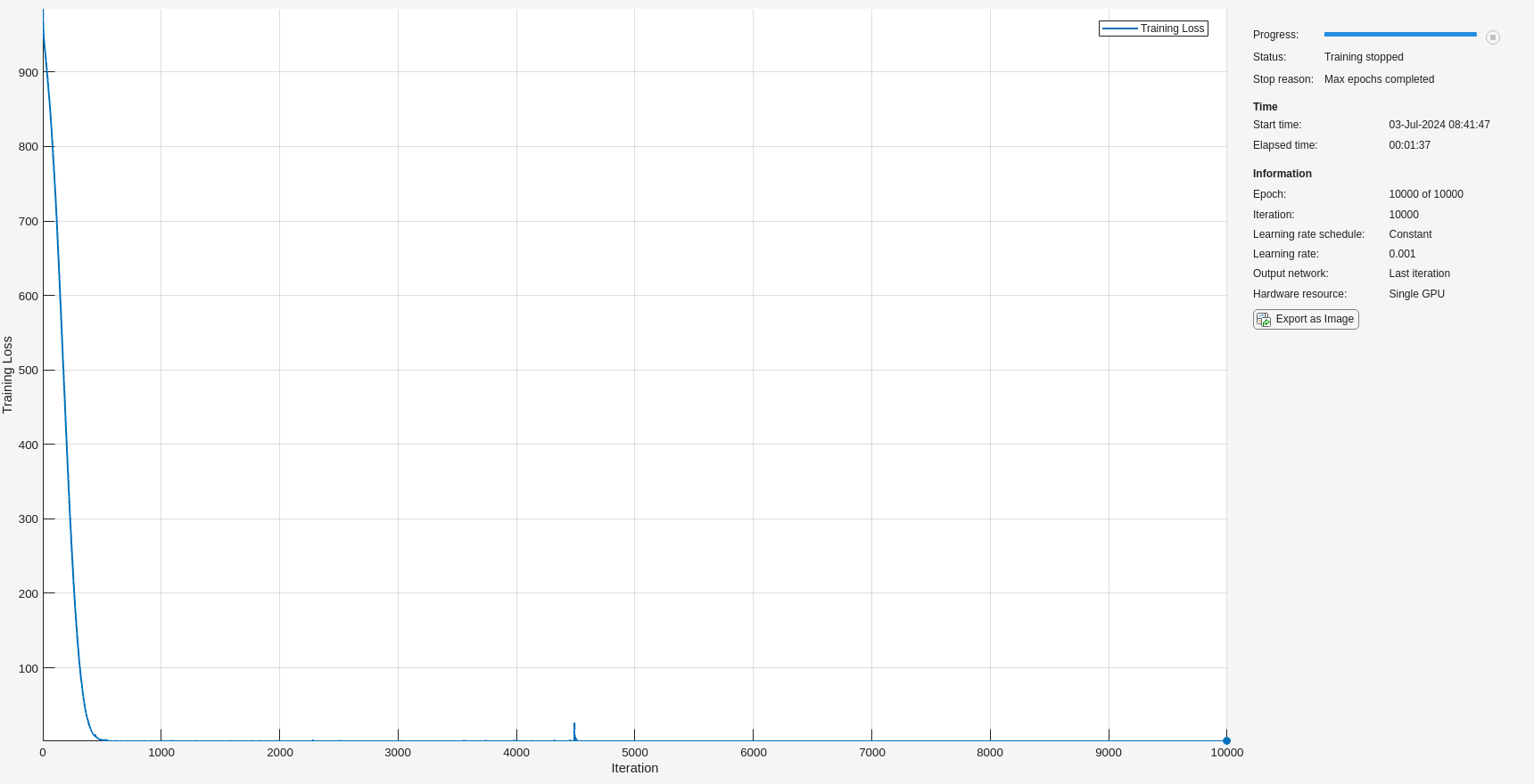
Train the Network
You can use the pretrained network to run the example without having to wait for training. To reduce training time, trainList is set to 1 to train only the network corresponding to the first moment (ZH). To train networks of other moments, include the corresponding numbers 1-6 in trainList.
trainList = [1];
netList = cell(1,Nmoments);
for cc = 1:Nmoments
    if ismember(cc, trainList)
        opts = trainingOptions("adam", ...
            MaxEpochs=10000, ...
            MiniBatchSize=40, ...
            InitialLearnRate=1e-3, ...
            Verbose=false, ...
            Plots="training-progress", ...
            ExecutionEnvironment="auto");
        net = trainnet(imgs(:,:,cc,trainSet),resps(:,:,cc,trainSet),dlnet,"mse",opts);
    else
        load("CNN_Net_"+cc+".mat");
    end
    netList{cc} = net;
end
Evaluate the Network
Now that the network is trained, obtain the CNN output of the test dataset and display the RMSE of the CNN output compared to the NEXRAD ground truth.
predOut = zeros(Nazimuth,Ngates,Nmoments,numel(testSet));
for cc = 1:Nmoments
    predOut(:,:,cc,:) = minibatchpredict(netList{cc},imgs(:,:,cc,testSet));
end
helperErrorStatistics(predOut,resps(:,:,:,testSet));
    MomentName    RMSE_Avg    Specification       Unit
    __________    ________    _____________    __________

    {'ZH'   }       1.09             1         {'dB'    }
    {'Vr'   }       0.33             1         {'m/s'   }
    {'SW'   }       0.34             1         {'m/s'   }
    {'ZDR'  }       0.24           0.2         {'dB'    }
    {'Rhohv'}      0.007          0.01         {'N/A'   }
    {'Phidp'}       1.71             2         {'degree'}
As shown in the table above, the RMSE of the CNN estimates for all the 6 radar moments is lower than that of the PPP estimates and either meets or nearly meets the data quality specifications of NEXRAD. As a comparison, weather radar images of CNN estimates for the first test case minus corresponding ground truth are also plotted. As can be seen, all the images look less noiser, which indicate CNN estimates are closer to the NEXRAD truth than the PPP estimates.
helperImagePlot(range,azimuth,predOut(:,:,:,1)-resps(:,:,:,testSet(1)),'CNN Estimates minus Ground Truth',1);
Also, the histogram of CNN estimates minus the NEXRAD truth of each radar moment is plotted, which shows all the CNN estimates have a narrower range of estimation error than PPP estimates.
helperHistPlot(predOut(:,:,:,1),resps(:,:,:,testSet(1)),'Histogram of CNN Estimates minus Truth');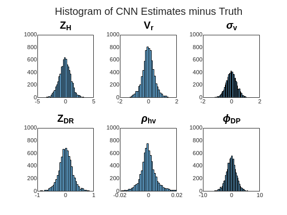
The reason why CNN could improve the radar moment estimation is that CNN utilizes spatial information of the input images, which was not included by the PPP method that estimates radar moments at a single range gate. Also, if more training and testing datasets are used, the RMSE of CNN estimates is expected to improve further.
Summary
This example showed how to simulate time series data from the NEXRAD Level-II data. RMSE, visual comparison, and histograms showed the CNN can be used to improve the accuracy of weather radar moment estimation. With this example, you can further explore the simulated weather time series data to evaluate various signal processing algorithms for weather radar.
References
[1] Zhang, G. Weather Radar Polarimetry. Boca Raton: CRC Press, 2016.
[2] Li, Z, et al. "Polarimetric phased array weather radar data quality evaluation through combined analysis, simulation, and measurements," IEEE Geosci. Remote Sens. Lett., vol. 18, no. 6, pp. 1029–1033, Jun. 2021.
Supporting Functions
helperPulsePairProcessing
function moment = helperPulsePairProcessing(Vh,Vv,lambda,prf)
    % Apply Pulse-Pair-Processing for radar moment estimation
    % Vh and Vv are N-by-M matrices, where N is the number of resolution cells,
    % and M is the number of pulses per trial.
    np = size(Vh,2);
    prt = 1/prf;

    % Covariance matrix
    R0_hh = mean(abs(Vh.^2),2);
    R0_vv = mean(abs(Vv.^2),2);
    C0_hv = mean(conj(Vh).*Vv,2);
    R1_hh = mean(conj(Vh(:,1:np-1)).*(Vh(:,2:np)),2);

    % Pulse-Pair-Processing
    moment.Pr = pow2db(R0_hh);
    moment.Vr = -lambda/(4*pi*prt)*angle(R1_hh);
    moment.SW = abs(lambda/(4*pi*prt).*(2*log(abs(R0_hh)./abs(R1_hh))).^0.5);
    moment.ZDR = pow2db(R0_hh./R0_vv);
    moment.Rhohv = abs(C0_hv)./(R0_hh).^0.5./(R0_vv).^0.5;
    moment.Phidp = fusion.internal.units.interval(angle(C0_hv)*180/pi,[0,360]);
end
helperImagePlot
function helperImagePlot(range,azimuth,data,sharedTitle,flag)
    % Display radar images in a tiled chart layout
    [rr,aa] = meshgrid(range/1e3,azimuth);
    [xx,yy] = pol2cart(deg2rad(aa),rr);
    f = figure;
    f.Position=[0 0 2000 1000];
    t = tiledlayout(2,3);
    % ZH
    nexttile
    helperSectorPlot(xx,yy,data(:,:,1),'ZH',flag);
    title('Z_{H}');
    % Vr
    nexttile
    helperSectorPlot(xx,yy,data(:,:,2),'Vr',flag);
    title('V_{r}');
    % SW
    nexttile
    helperSectorPlot(xx,yy,data(:,:,3),'SW',flag);
    title('\sigma_{v}');
    % ZDR
    nexttile
    helperSectorPlot(xx,yy,data(:,:,4),'ZDR',flag);
    title('Z_{DR}');
    % Rhohv
    nexttile
    helperSectorPlot(xx,yy,data(:,:,5),'Rhohv',flag);
    title('\rho_{hv}');
    % Phidp
    nexttile
    helperSectorPlot(xx,yy,data(:,:,6),'Phidp',flag);
    title('\phi_{DP}');
    % Shared title
    title(t,sharedTitle);
end
helperSectorPlot
function helperSectorPlot(xx,yy,data,varName,flag)
    % Plot plan position indicator (PPI) images
    pcolor(xx,yy,data);
    shading flat
    axis tight
    colormap('jet');
    colorbar;
    xlabel('Zonal Distance (km)');
    ylabel('Meridional Distance (km)');
    xlim([0 50]);
    ylim([0 50]);
    grid on;
    switch varName
      case 'ZH'
        if flag == 0
            cmin = 0;
            cmax = 70;
        else
            cmin = -5;
            cmax = 5;
        end
        clim([cmin,cmax]);
        c = colorbar;
        c.Label.String = 'dBZ';
        title('Z_{H}');
      case 'Vr'
        if flag == 0
            cmin = -25;
            cmax = 25;
        else
            cmin = -2;
            cmax = 2;
        end
        clim([cmin,cmax]);
        c = colorbar;
        c.Label.String = 'm/s';
        title('V_{r}');
      case 'SW'
        if flag == 0
            cmin = 0;
            cmax = 10;
        else
            cmin = -2;
            cmax = 2;
        end
        clim([cmin,cmax]);
        c = colorbar;
        c.Label.String = 'm/s';
        title('\sigma_{v}');
      case 'ZDR'
        if flag == 0
            cmin = -6;
            cmax = 6;
        else
            cmin = -1;
            cmax = 1;
        end
        clim([cmin,cmax]);
        c = colorbar;
        c.Label.String = 'dB';
        title('Z_{DR}');
      case 'Rhohv'
        if flag == 0
            cmin = 0.8;
            cmax = 1.0;
        else
            cmin = -0.02;
            cmax = 0.02;
        end
        clim([cmin,cmax]);
        title('\rho_{hv}');
      case 'Phidp'
        if flag == 0
            cmin = 0;
            cmax = 360;
        else
            cmin = -10;
            cmax = 10;
        end
        clim([cmin,cmax]);
        c = colorbar;
        c.Label.String = 'degree';
        title('\phi_{DP}');
      otherwise
        colormap([0 0 0;0 1 0]);
    end
end
helperHistPlot
function helperHistPlot(estimate,truth,sharedTitle)
    % Plot histograms of estimate minus truth
    [Naz,Ngates,Nchan,~] = size(estimate);
    data = zeros(Naz,Ngates,Nchan);
    for ii = 1:Nchan
        data(:,:,ii) = estimate(:,:,ii)-truth(:,:,ii);
    end
    figure;
    t = tiledlayout(2,3);
    % ZH
    nexttile
    histogram(data(:,:,1));
    xlim([-5 5])
    ylim([0 1000])
    title('Z_{H}','FontSize',15);
    % Vr
    nexttile
    histogram(data(:,:,2));
    xlim([-2 2])
    ylim([0 1000])
    title('V_{r}','FontSize',15);
    % SW
    nexttile
    histogram(data(:,:,3));
    xlim([-2 2])
    ylim([0 1000])
    title('\sigma_{v}','FontSize',15);
    % ZDR
    nexttile
    histogram(data(:,:,4));
    xlim([-1 1])
    ylim([0 1000])
    title('Z_{DR}','FontSize',15);
    % Rhohv
    nexttile
    histogram(data(:,:,5));
    xlim([-0.02 0.02])
    ylim([0 1000])
    title('\rho_{hv}','FontSize',15);
    % Phidp
    nexttile
    histogram(data(:,:,6));
    xlim([-10 10])
    ylim([0 1000])
    title('\phi_{DP}','FontSize',15);
    % Shared title
    title(t,sharedTitle,'FontSize',15);
end
helperErrorStatistics
function helperErrorStatistics(estimate,truth)
    % Calculate averaged RMSE of estimate compared to truth
    Nchan = size(estimate,3);
    Nimages = size(estimate,4);
    RMSE_moment = zeros(Nimages,Nchan);
    for ii = 1:Nimages
        for jj = 1:Nchan
            RMSE_moment(ii,jj) = rmse(estimate(:,:,jj,ii),truth(:,:,jj,ii),'all','omitnan');
        end
    end
    RMSE_Avg = [round(mean(RMSE_moment(:,1)),2);round(mean(RMSE_moment(:,2)),2);round(mean(RMSE_moment(:,3)),2);...
        round(mean(RMSE_moment(:,4)),2);round(mean(RMSE_moment(:,5)),3);round(mean(RMSE_moment(:,6)),2)];
    MomentName = {'ZH';'Vr';'SW';'ZDR';'Rhohv';'Phidp'};
    Specification = [1;1;1;0.2;0.01;2];
    Unit = {'dB';'m/s';'m/s';'dB';'N/A';'degree'};
    T = table(MomentName,RMSE_Avg,Specification,Unit);
    disp(T);
end