Introduction to Pulse Integration and Fluctuation Loss in Radar
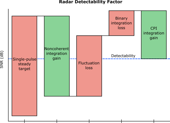
The radar detectability factor is the minimum signal-to-noise ratio (SNR) required to declare a detection with the specified probabilities of detection, , and false alarm, . The Modeling Radar Detectability Factors example discusses in detail the computation of the detectability factor for a radar system given a set of performance requirements. It shows how to use the detectability factor in the radar equation to evaluate the maximum detection range. It also shows how to compute the effective probability of detection at a given range.
Typically, when a radar detectability factor is computed for pulses received from a Swerling target, it already includes the pulse integration gain assuming noncoherent integration and a fluctuation loss due to the target radar cross section (RCS) fluctuation. However, if other pulse integration techniques are used, such as binary or cumulative, an additional integration loss must be added to the detectability factor. Similarly, if the system employs diversity, the target RCS fluctuation can be exploited to achieve a diversity gain.
This example illustrates how to compute the pulse integration loss for several pulse integration techniques. It also shows computation of the losses due to the target's RCS fluctuation.
Pulse Integration
Typically, in a pulsed radar the required detection performance cannot be achieved with a single pulse. Instead, pulse integration is used to improve the SNR by adding signal samples together while averaging out the noise and interference.
Coherent and Noncoherent Integration
In coherent integration the complex signal samples are combined after coherent demodulation. Given that the samples are added in phase, the coherent integration process increases the available SNR by the number of integrated pulses, . However, coherent integration might not always be possible due to the target's RCS fluctuation, which can make the coherent processing interval (CPI) too short to collect enough samples.
Noncoherent integration discards the phase information and combines the squared magnitudes (assuming the square-law detector) of the signal samples instead. Since the phase information is lost in this case, the integration gain of noncoherent integration is lower than that of coherent integration given the same number of received pulses. In addition, unlike the coherent integration gain, the gain from the noncoherent integration is also a function of and . Examine how sensitive is the noncoherent integration gain to these parameters and compare it to the coherent integration gain.
Compute the integration gain as a function of the number of pulses for several different values of and .
% Number of received pulses
N = 1:100;

% Detection probability
Pd = [0.5 0.95];

% Probability of false alarm
Pfa = [1e-4 1e-8];
The noncoherent integration gain, , can be defined as a difference (in dB) between a single-pulse detectability factor, , and an -pulse detectability factor, , both computed for a steady target ("0" subscript indicates the steady target i.e. the Swerling 0 case)
[1].
% Single-pulse detectability factor
D0 = detectability(Pd,Pfa,1);

numPdPfa = numel(Pd)*numel(Pfa);

% N-pulse detectability
D0n = zeros(numPdPfa,numel(N));

for i = 1:numel(N)
    D0n(:,i) = reshape(detectability(Pd,Pfa,N(i)),[],1);
end

% Noncoherent integration gain
Gnc = reshape(D0,[],1)-D0n;
The coherent integration gain does not depend on and , and simply equals the number of integrated pulses.
% Coherent integration gain
Gc = pow2db(N);
We plot the computed gains on a single plot together with a line, which is a commonly used approximation for the noncoherent gain.
figure
semilogx(N,Gnc(1:2,:),'LineWidth',2)
hold on
semilogx(N,Gnc(3:4,:),'--','LineWidth',2)
semilogx(N,Gc,'k','LineWidth',2)
semilogx(N,pow2db(sqrt(N)),'k:','LineWidth',2)

xlabel('Number of Integrated Pulses')
ylabel('Gain (dB)')
title('Pulse Integration Gain')

labels = helperLegendLabels('Noncoherent P_d=%.2f','P_{fa}=%.0e',Pd,Pfa);
labels{end + 1} = 'Coherent';
labels{end + 1} = 'N^{1/2}';

xticks = [1 2 5 10 20 50 100];
set(gca(),'xtick',xticks,'xticklabel',num2cell(xticks))
legend(labels,'location','best')
grid on

yyaxis(gca(),'right')
set(gca(),'ycolor','k')
ylabel('Exponent of N')
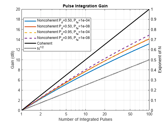
From this result you can observe that the noncoherent integration gain is not very sensitive to and . It also appears to be significantly higher than the approximation with the actual values being between and [1, 2].
Binary Integration
Binary integration, also known as the M-of-N integration, is a double-threshold system. The first threshold is applied to each pulse resulting in detection outcomes each with a probability of detection, , and false alarm, . These outcomes are then combined and compared to the second threshold. If at least out of pulses cross the first threshold, a target is declared to be present. Given the detection and the false alarm probabilities of the individual outcomes, the resultant and after the binary detection are
Thus, the desired can be achieved starting with a significantly lower detection probability in a single detection. Similarly, the single pulse could be set to a higher value than the required . For ,, , and determine the probabilities of detection and false alarm for each individual detection.
[~,pd,pfa] = binaryintloss(0.95,1e-8,4,2)
pd =
0.7514
pfa =
4.0826e-05
Since binary integration is suboptimal, it results in a binary integration loss compared to the optimal noncoherent integration. For a given set of , , and this loss depends on the choice of . However, the optimal value of is not a sensitive selection and it can be different from the optimum without significant penalty. For a nonfluctuating target, a good choice of was shown to be [3].
Compute the binary integration loss as a function of for several values of and .
% Binary integration loss
Lb = zeros(numPdPfa,numel(N));

for i = 1:numel(N)
    Lb(:,i) = reshape(binaryintloss(Pd,Pfa,N(i)),[],1);
end

figure
semilogx(N,Lb,'LineWidth',2)

xlabel('Number of Integrated Pulses')
ylabel('Loss (dB)')
title({'Binary Integration Loss','M=0.955N^{0.8}'})

set(gca(),'xtick',xticks,'xticklabel',num2cell(xticks))
labels = helperLegendLabels('P_d=%.2f','P_{fa}=%.0e',Pd,Pfa);
legend(labels,'location','best')
grid on
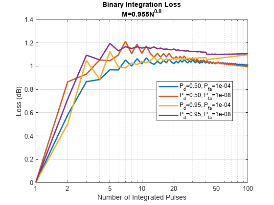
The resultant loss is around 1 to 1.2 dB and is not very sensitive to , , and . The binary integrator is a relatively simple automatic detector. It is also robust to non-Gaussian background noise and clutter.
M-of-N Integration Over Multiple CPIs
M-of-N integration scheme can also be applied to multiple CPIs or multiple scans. This might be necessary when detecting high-velocity targets that can move across several resolution cells during the integration time. In this case, pulses are divided into groups, where is the number of CPIs. Within each CPI, pulses can be coherently or noncoherently integrated resulting in probabilities of detection, , and false alarm, . The target is declared to be present if it was detected in at least CPIs out of . The detectability factor for M-of-N integration assuming required and is computed here as a function of the total number of pulses, , for several choices of the M-of-N threshold.
% M-of-N detection thresholds: 1-of-2, 2-of-3, and 1-of-3
n = [2 3 3];
m = [1 2 1];

% Detectability factor for M-of-N CPI integration
Dmn = zeros(numel(n),numel(N));

for i = 1:numel(n)
    % Detection and false alarm probabilities required in a single CPI
    [~,pd,pfa] = binaryintloss(Pd(2),Pfa(2),n(i),m(i));

    for j = 1:numel(N)
        Dmn(i,j) = detectability(pd,pfa,N(j)/n(i));
    end
end
The resultant loss is the difference (in dB) between the SNR required when M-of-N integration is performed over CPIs and the SNR required when all pulses are processed within a single CPI.
.
% M-of-N integration loss with respect to the optimal noncoherent
% integration
Lmn = Dmn-D0n(4,:);

figure
semilogx(N,Lmn,'LineWidth',2)

xlabel('Number of Integrated Pulses')
ylabel('Loss (dB)')
title({'Loss for M-of-N Integration over Multiple CPIs',sprintf('P_d=%.2f, P_{fa}=%.0e',Pd(2),Pfa(2))})

set(gca(),'xtick',xticks,'xticklabel',num2cell(xticks))

labels = arrayfun(@(i)sprintf('%d-of-%d',m(i),n(i)), 1:numel(n),'UniformOutput',false);
legend(labels,'location','south')
grid on
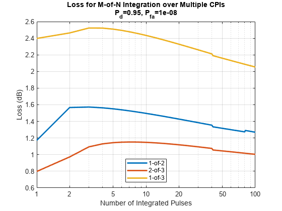
This result shows that the loss is sensitive to the chosen M-of-N threshold, and that it tends to decrease with , although the variation with the number of pulses is not very strong.
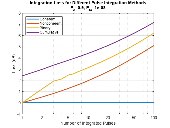
The results above compute the integration loss with respect to optimal noncoherent integration. Alternatively, different integration methods can be compared with respect to coherent integration. Compare noncoherent integration, binary integration, and a special case of the M-of-N integration with (called cumulative integration) for and .
Compute the detectability factor for the coherent case assuming a single pulse is detected in the envelope detector after integrating pulses coherently.
% Detectability factor for coherent integration
Dc = detectability(Pd(2),Pfa(2),1) - 10*log10(N);
Then compute the losses for different integration types with respect to coherent integration.
% Noncoherent integration loss
Li = D0n(4,:)-Dc;

%  Binary integration loss
Lbi = D0n(4,:)-Dc+Lb(4,:);

% Cumulative integration loss with 1-of-3 detection
Lcum = D0n(4,:)-Dc+Lmn(3,:);
Plot and compare these integration losses for different values of the total number of integrated pulses.
figure
semilogx(N,zeros(size(Dc)),'LineWidth',2)
hold on
semilogx(N,Li,'LineWidth',2)
semilogx(N,Lbi,'LineWidth',2)
semilogx(N,Lcum,'LineWidth',2)

xlabel('Number of Integrated Pulses')
ylabel('Loss (dB)')
title({'Integration Loss for Different Pulse Integration Methods',sprintf('P_d=%.1f, P_{fa}=%.0e',Pd(2),Pfa(2))});

set(gca(),'xtick',xticks,'xticklabel',num2cell(xticks))
legend({'Coherent','Noncoherent','Binary','Cumulative'},'location','northwest')
ylim([-1 8])
grid on
Fluctuation Loss
Since the RCS of a real-world target fluctuates, the signal energy required to achieve a given probability of detection is higher compared to that required for a steady target. This increase in the energy is the fluctuation loss. Evaluate the fluctuation loss as a function of the probability of detection for different values of and .
% Detection probability
Pd = linspace(0.01,0.995,100);

% Probability of false alarm
Pfa = [1e-8 1e-4];

% Number of received pulses
n = [1 10 50];
The fluctuation loss can be computed as a difference (in dB) between the detectability factor for the fluctuating target, , and the detectability factor for the steady target,
where the subscript indicates the Swerling case [1]. This example performs the computation for Swerling 1 and Swerling 2 cases that model slow and fast fluctuating targets, respectively.
% Fluctuation loss for Swerling 1 case
L1f = zeros(numel(Pd),numel(Pfa),numel(n));

% Fluctuation loss for Swerling 2 case
L2f = zeros(numel(Pd),numel(Pfa),numel(n));

for i = 1:numel(n)
    % Detectability factor for a steady target
    D0n = detectability(Pd,Pfa,n(i),'Swerling0');

    % Detectability factor for Swerling 1 case fluctuating target
    D1n = detectability(Pd,Pfa,n(i),'Swerling1');

    % Detectability factor for Swerling 2 case fluctuating target
    D2n = detectability(Pd,Pfa,n(i),'Swerling2');

    L1f(:,:,i) = D1n-D0n;
    L2f(:,:,i) = D2n-D0n;
end
The computed fluctuation loss is plotted here against the probability of detection. This result shows that in the Swerling 1 case, when there is no pulse-to-pulse RCS fluctuation, the loss is not very sensitive to the number of pulses. However, it is very sensitive to the probability of detection. High values of the required result in a large fluctuation loss. In the case of the Swerling 2 model, the RCS fluctuates from pulse-to-pulse, therefore the fluctuation loss is very sensitive to the number of pulses and decreases rapidly with The fluctuation loss is not a strong function of in both Swerling 1 and 2 cases.
figure
ax1 = subplot(1,2,1);
helperPlotFluctuationLoss(ax1,Pd,L1f)

title(ax1,{'Fluctuation Loss','Swerling 1 Case'});
labels = helperLegendLabels('N=%d','P_{fa}=%.0e',n,Pfa);
legend(labels)

ax2 = subplot(1,2,2);
helperPlotFluctuationLoss(ax2,Pd,L2f)

title(ax2,{'Fluctuation Loss','Swerling 2 Case'})
legend(labels)

set(gcf,'Position',[100 100 800 600])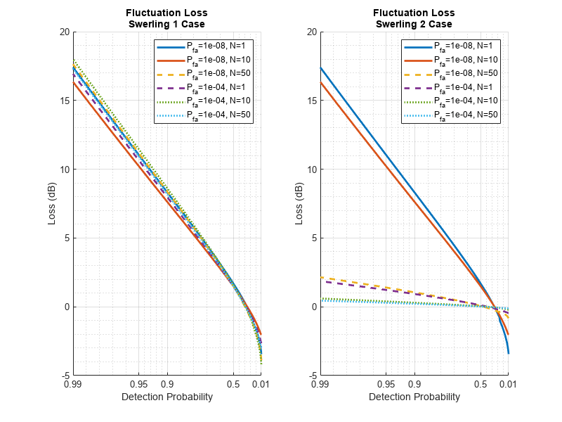
Diversity Gain
The Swerling 2 case can also be used to represent target samples obtained by a radar system with diversity (for example, frequency, space, polarization, among others). As was shown in the earlier section, the fluctuation loss decreases with the number of received pulses for a Swerling 2 target. This indicates that obtaining more samples with diversity can reduce the fluctuation loss. Consider pulses received during a dwell time. These pulses might be integrated coherently to provide a single pulse at the input to the envelope detector. However, if the radar system can transmit at different frequencies, pulses could be transmitted in groups of . For example, if a radar system transmits a total of pulses, they could be transmitted in two groups of eight, four groups of four, eight groups of two, or all 16 pulses at different frequencies.
% Total number of transmitted pulses
N = 16;

% Number of diversity samples
M = [1 2 4 8 16];
Within each frequency group coherent integration can be applied to the received pulses providing diverse samples, which then can be aggregated by noncoherent integration. If the frequencies are chosen such that the echoes at different frequencies are decorrelated, there is going to be an optimal number of diversity samples that minimizes the required signal energy. Assume the following values for the required and .
% Detection probability
Pd = [0.9 0.7 0.5];

% Probability of false alarm
Pfa = 1e-6;
To provide the required detection performance, the energy in each diversity sample must be equal to . Since the pulses within each group are coherently integrated, the required SNR for each pulse equals .
% Detectability factor
D = zeros(numel(Pd),numel(M));

for i = 1:numel(M)
    D(:,i) = detectability(Pd,Pfa,M(i),'Swerling2') - 10*log10(N/M(i));
end
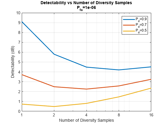
The following plot shows the detectability factor as a function of the number of diversity samples. From this result you can see that for each value of there is an optimal value of For example, when is 0.9, the best result is achieved when transmitting eight groups of two pulses. The detectability factor in this case is almost 5 dB lower than when all 16 pulses are integrated coherently. This is a diversity gain due to utilizing multiple frequencies.
figure
semilogx(M,D,'LineWidth',2)

ylabel('Detectability (dB)')
xlabel('Number of Diversity Samples')
title({'Detectability vs Number of Diversity Samples',sprintf('P_{fa}=%.0e',Pfa)})

set(gca(),'xtick',M,'xticklabel',num2cell(M))
legend(helperLegendLabels('P_{d}=%.1f',Pd))
grid on
Conclusion
This example discusses pulse integration and fluctuation losses included in the effective detectability factor. It starts by introducing coherent, noncoherent, binary, and cumulative pulse integration techniques and examines how the resulting integration loss depends on the detection parameters, that is, the probability of detection, probability of false alarm, and the number of received pulses. The fluctuation loss is discussed next. The example shows that in the case of a slowly fluctuating target the required high detection probability results in the large fluctuation loss, while changes in the false alarm and the number of received pulses have a much lesser impact. On the other hand, the fluctuation loss in the case of a rapidly fluctuating target decreases rapidly with the number of received pulses. It is then shown that the RCS fluctuation together with the frequency diversity can be employed to achieve a diversity gain.
References
Barton, David Knox. Radar Equations for Modern Radar. Artech House, 2013.
Richards, M. A. "Noncoherent integration gain, and its approximation." Georgia Institute of Technology, Technical Memo (2010).
Richards, M. A. Fundamentals of Radar Signal Processing. Second edition, McGraw-Hill Education, 2014.