Maritime Clutter Suppression with Neural Networks

Since R2022b

This example uses:

This example shows how to train and evaluate neural networks to suppress maritime clutter returns from radar images using the Deep Learning Toolbox™. The Deep Learning Toolbox provides a framework for designing and implementing deep neural networks with algorithms, pretrained models, and apps.

Two example scenarios are shown here. In the first scenario, a denoising convolutional neural network (CNN) is used to suppress clutter in a plan position indicator (PPI) image. The Simulate a Maritime Radar PPI example demonstrates how to use Radar Toolbox™ to create PPI images for a rotating radar at sea. In the second scenario, a convolutional autoencoder is used to suppress clutter in a range-time image. The Simulate a Coastal Surveillance Radar example shows how to use Radar Toolbox to create range-time images for a stationary coastal surveillance radar.

Scenario 1: Clutter Suppression for a Maritime Radar PPI

In this first scenario, a rotating radar on a tall platform in open water has been simulated to create PPI radar images with clutter and target returns. A denoising convolutional network is used to suppress the clutter returns.

Set the random seed for repeatability.

rng default

The Maritime Radar PPI Dataset

The dataset contains 84 pairs of synthetic radar images. Each pair consists of an input image, which has both sea clutter and extended target returns, and a desired response image, which includes only the target returns. The images were created using a radarScenario simulation with a radarTransceiver and a rotating uniform linear array (ULA). Each image contains two nonoverlapping cuboid targets with one representing a small container ship and the other representing a larger container ship.

The following parameters are fixed from image to image:

Frequency (10 GHz)
Pulse length (80 ns)
Range resolution (7.5 m)
PRF (1 kHz)
Azimuth beamwidth (1 deg)
Radar height (55 m)
Rotation rate (50 RPM)
Small target dimensions (120-by-18-by-22 m)
Large target dimensions (200-by-32-by-58 m)
Small target fixed RCS (30 dBsm)
Large target fixed RCS (40 dBsm)

The following parameters are randomized from image to image:

Wind speed (7 to 17 m/s)
Wind direction (0 to 180 deg)
Target position (anywhere on the sea surface)
Target heading (0 to 360 deg)
Target speed (4 to 19 m/s)

This variation ensures that a network trained on this data will be applicable to a fairly wide range of target profiles and sea states for this radar configuration. For more information on sea states, see the Maritime Radar Sea Clutter Modeling example.

Download the Maritime Radar PPI Images dataset and unzip the data and license file into the current working directory.

dataURL = 'https://ssd.mathworks.com/supportfiles/radar/data/MaritimeRadarPPI.zip';
unzip(dataURL)

Load the image data and pretrained network into a struct called imdata. This struct will have fields img1 through img84 and resp1 through resp84.

imdata = load('MaritimeRadarPPI.mat');

Prepare the Data

You can use the pretrained network to run the example without having to wait for training. Set the doTrain variable to true by selecting the check box below to perform the training steps. The training for this network takes less than 2 minutes on an NVIDIA Titan RTX™ GPU.

doTrain = false;
if ~doTrain
    load PPIDeclutterNetwork.mat %#ok<UNRCH>
end

Image sets 1-70 are used for training and 71-80 for validation. The last 4 images will be used for evaluation of the network.

Format the data as a 4D array for use with the network trainer and training options. The first two dimensions are considered spatial dimensions. The third dimension is for channels (such as color channels). The separate images are arranged along the 4th dimension. The cluttered inputs are simply referred to as images, and the desired output is known as the response. Single precision is used since that is native to the neural network trainer.

imgs  = zeros(626,626,1,84,'single');
resps = zeros(626,626,1,84,'single');
for ind = 1:84
   imgs(:,:,1,ind) = imdata.(sprintf('img%d',ind));
   resps(:,:,1,ind) = imdata.(sprintf('resp%d',ind));
end

After formatting, clear the loaded data struct to save RAM.

clearvars imdata

Network Architecture

A network is defined by a sequence of layer objects. An imageInputLayer is used as the input layer so that the images may be used without any reformatting. A cascade of 2D convolution layers with normalizations and nonlinear activations is used for the hidden layers.

Create the input layer. Specify the spatial size of the input images along with the number of channels, which is 1.

layers = imageInputLayer([626 626 1]);

Add 3 sets of convolution+normalization+activation. Each convolution layer consists of a set of spatial filters. The batchNormalizationLayer biases and scales each mini batch to improve numerical robustness and speed up training. The leakyReluLayer is a nonlinear activation layer that scales values below 0 while leaving values greater than 0 unmodified.

Care must be taken to ensure the spatial and channel dimensions are consistent from layer to layer and that the size and number of channels of the output from the last layer matches the size and number of channels of the desired response images. Set the Padding property of the convolution layers to 'same' so that the filtering process does not change the spatial size of the images.

layers = [layers;

          % Set 1: Convolution + Normalization + Activation
          convolution2dLayer([5 5],1,Padding='same');
          batchNormalizationLayer;
          leakyReluLayer(0.2);

          % Set 2: Convolution + Normalization + Activation
          convolution2dLayer([6 6],4,Padding='same');
          batchNormalizationLayer;
          leakyReluLayer(0.2);

          % Set 3: Convolution + Normalization + Activation
          convolution2dLayer([5 5],1,Padding='same');
          batchNormalizationLayer;
          leakyReluLayer(0.2)];

Train the Network

Use the trainingOptions function to configure how the network is trained. This provides control over things like learn-rate scheduling and the size of mini batches, in addition to specifying the training method to use. The trainingOptions can also be used to specify a validation data set, which is used to determine the running performance. This also provides a way to return the network at whichever iteration yielded the lowest validation error, since the performance of a network may not improve monotonically with iterations.

Define the indices of the sets to use for training and for validation.

trainSet = 1:70;  % Training set
valSet   = 71:80; % Validation set

Now create the trainingOptions. Use the adaptive moment estimation (Adam) solver. Train for a maximum of 80 epochs with a mini batch size of 20. Set the initial learn rate to 0.1. The validation set is specified with a 1-by-2 cell array containing the validation image and response arrays. Set the ValidationFrequency to 25 to evaluate the loss for the validation set every 25 iterations. Specify OutputNetwork as 'best-validation' to return the network at the iteration that had the least validation loss. Set Verbose to true to print the training progress.

opts = trainingOptions('adam', ...
    Metrics='rmse', ...
    MaxEpochs=80, ...
    MiniBatchSize=20, ...
    Shuffle='every-epoch', ...
    InitialLearnRate=0.1, ...
    ValidationData={imgs(:,:,:,valSet),resps(:,:,:,valSet)}, ...
    ValidationFrequency=25, ...
    OutputNetwork='best-validation', ...
    Verbose=true);

Training is initiated by using trainnet. Input the 4D training image and response arrays, the vector of network layers, and the training options. Specify the loss function as the mse function, which computes the half mean squared error. This section will only run if the doTrain flag is set to true.

A compatible GPU is used by default if available. Using a GPU requires Parallel Computing Toolbox™ and a supported GPU device. For information on supported devices, see GPU Computing Requirements (Parallel Computing Toolbox). Otherwise, trainnet uses the CPU.

if doTrain
    [net1,info] = trainnet(imgs(:,:,:,trainSet),resps(:,:,:,trainSet),layers,@mse,opts);

Use the provided helper function to plot the training and validation loss on a log scale.

    helperPlotTrainingProgress(info)
end

    Iteration    Epoch    TimeElapsed    LearnRate    TrainingLoss    ValidationLoss    TrainingRMSE    ValidationRMSE
    _________    _____    ___________    _________    ____________    ______________    ____________    ______________
            0        0       00:00:01          0.1                        0.00012283                        2.5038e-05
            1        1       00:00:01          0.1      1.1592e+05                           0.76918                  
           25        9       00:00:09          0.1          308.52             146.9        0.039681          0.027381
           50       17       00:00:15          0.1          51.686            48.675        0.016241          0.015761
           75       25       00:00:22          0.1          2.4393            2.2141       0.0035283         0.0033615
          100       34       00:00:29          0.1        0.055494          0.084225      0.00053219        0.00065563
          125       42       00:00:36          0.1       0.0056642         0.0072286      0.00017002        0.00019207
          150       50       00:00:43          0.1      0.00075902        0.00074201       6.224e-05        6.1538e-05
          175       59       00:00:49          0.1      0.00038776        0.00016548      4.4486e-05        2.9062e-05
          200       67       00:00:56          0.1      0.00015933         9.961e-05      2.8516e-05        2.2547e-05
          225       75       00:01:02          0.1      0.00025666         9.283e-05      3.6192e-05        2.1766e-05
          240       80       00:01:06          0.1      0.00022196         9.109e-05      3.3657e-05        2.1561e-05
Training stopped: Max epochs completed

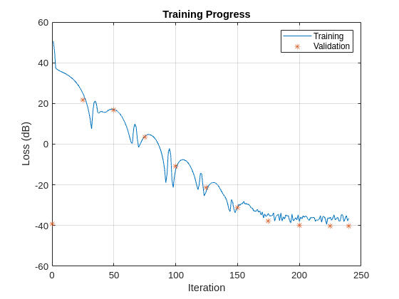
Figure contains an axes object. The axes object with title Training Progress, xlabel Iteration, ylabel Loss (dB) contains 2 objects of type line. One or more of the lines displays its values using only markers These objects represent Training, Validation.

The training and validation loss decreases steadily until an error floor is hit at around iteration 200. More training samples are needed to improve the performance of this network.

Evaluate the Network

Now that the network has been trained, use the last 4 images to evaluate the network.

evalSet = 81:84; % Evaluation set

Use the provided helper function to plot the input images alongside the responses output by the network. The results are normalized and pixels below -60 dB are clipped for easier comparison.

helperPlotEvalResults(imgs(:,:,:,evalSet),net1);

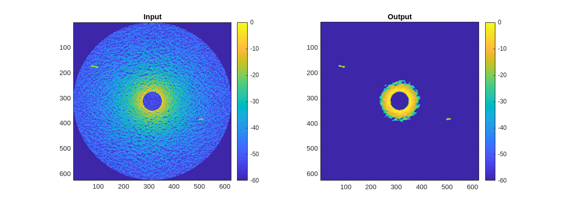
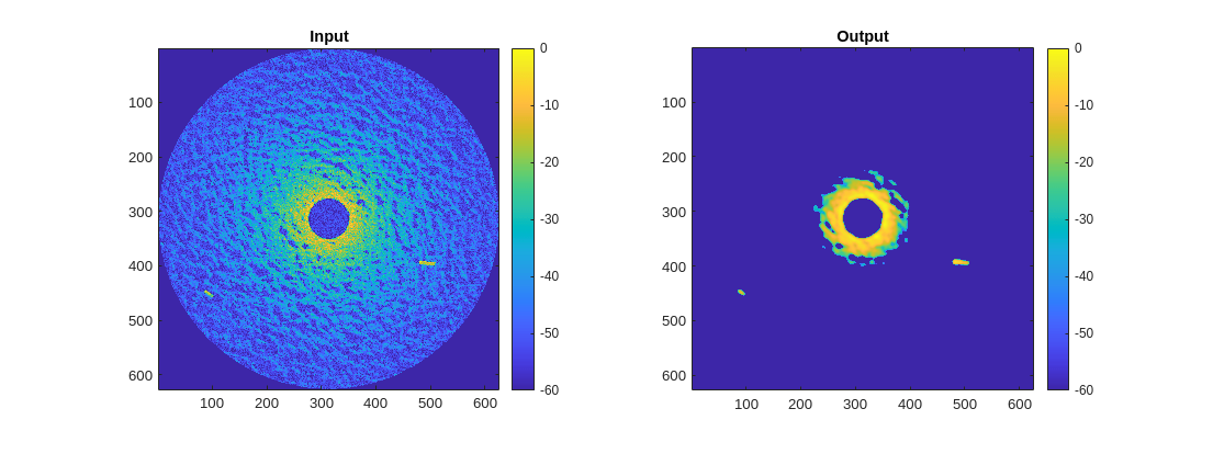
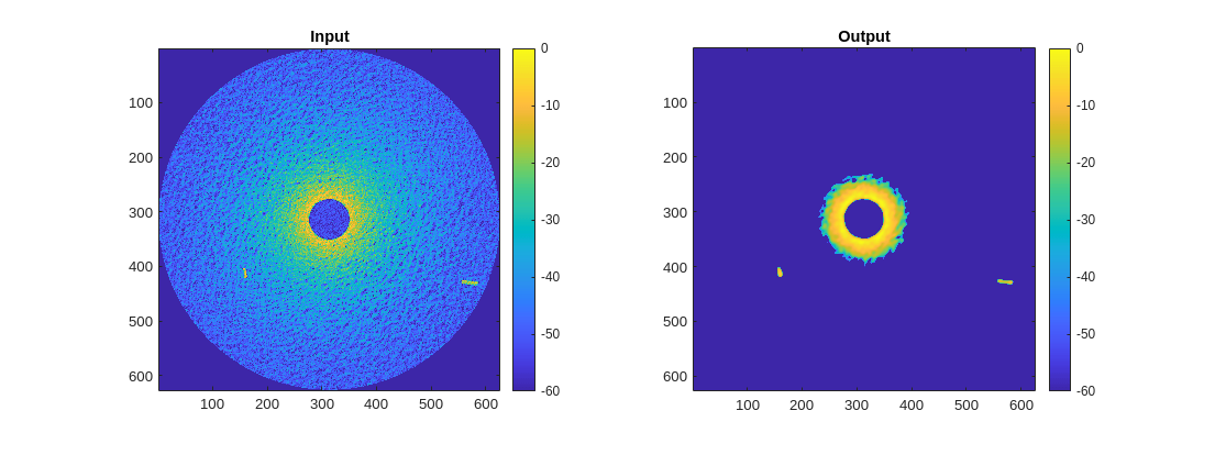
Figure contains 2 axes objects. Axes object 1 with title Input contains an object of type image. Axes object 2 with title Output contains an object of type image.

The network completely removes the sea clutter below a certain threshold of returned power while retaining the target signals with only a small dilation effect due to the size of the convolution filters used. The remaining high-power clutter near the center of the images could be removed by a spatially-aware layer, such as a fully-connected layer, or by preprocessing the original images to remove the range-dependent losses.

Scenario 2: Clutter Suppression for a Coastal Surveillance Radar

This section mitigates sea clutter for a stationary radar viewing moving targets at sea. A convolutional autoencoder is used to suppress the clutter returns.

Set the random seed for repeatability.

rng default

The Coastal Surveillance Radar Dataset

The dataset contains 10,000 pairs of synthetic range-time-intensity radar images. Each pair consists of an input image, which has both sea clutter and target returns, and a desired response image, which includes only the target returns. The images were created using a radarScenario simulation with a radarTransceiver and uniform linear array (ULA). Each image contains a single small extended target. A fairly high range resolution and a low PRF were used so that target range migration is visible. A short pulse is used for simplicity.

The following parameters are fixed from image to image:

Frequency (10 GHz)
Pulse length (21 ns)
Range resolution (3.2 m)
PRF (100 Hz)
Azimuth beamwidth (4 deg)
Number of pulses (80)
Number of range gates (80)
Radar height above sea surface (11 m)

The following parameters are randomized from image to image:

Sea state (1 to 5, proportional wind speeds from 3 to 13 m/s)
Target position (anywhere on the sea surface)
Target heading (0 to 360 deg)
Target speed (5 to 25 m/s)
Target RCS (-14 to 6 dBsm)
Target dimensions (length from 10 to 30 m, with proportional beam and height)

This variation ensures that a network trained on this data will be applicable to a fairly wide range of target profiles and sea states for this radar configuration.

Download the Coastal Surveillance Radar Images dataset and unzip the data and license file into the current working directory.

dataURL = 'https://ssd.mathworks.com/supportfiles/radar/data/CoastalSurveillanceRadarImages.zip';
unzip(dataURL)

Load the image data into a struct called imdata. This struct will have fields X and Y where X contains cluttered images and Y contains the ideal response images. Both are single-valued matrices of size 80-by-80-by-10,000 with each page representing an image. The images are formatted with fast-time (range) along the first dimension and slow-time (pulses) along the second dimension.

imdata = load('CoastalSurveillanceRadarImages.mat');

Prepare the Data

The data will be randomly segmented into a training set (80%), a validation set (10%), and an evaluation set (10%). Start by using helperSegmentData to get an index for each set.

numSets = size(imdata.X,3);
[trainIdx,valIdx,evalIdx] = helperSegmentData(numSets);

Format the sets into 1-by-2 cell arrays as expected by the network object.

trainData = {imdata.X(:,:,trainIdx), imdata.Y(:,:,trainIdx)};
valData   = {imdata.X(:,:,valIdx),   imdata.Y(:,:,valIdx)};
evalData  = {imdata.X(:,:,evalIdx),  imdata.Y(:,:,evalIdx)};

The network uses the 3rd dimension for channels and the 4th for different images, so swap the 3rd and 4th array dimensions now.

trainData = cellfun(@(t) permute(t,[1 2 4 3]),trainData,'UniformOutput',false);
valData   = cellfun(@(t) permute(t,[1 2 4 3]),valData,'UniformOutput',false);
evalData  = cellfun(@(t) permute(t,[1 2 4 3]),evalData,'UniformOutput',false);

Lastly, the data should be normalized for good training performance. Perform normalization on all of the training and validation input and output images using a column norm. Only the input images from the evaluation set need to be normalized. Save the scaling factor used for each column in each cluttered evaluation image so the normalization can be reversed on the output image for better comparison to the original.

trainData{1} = normalize(trainData{1},'norm');
trainData{2} = normalize(trainData{2},'norm');
valData{1}   = normalize(valData{1},'norm');
valData{2}   = normalize(valData{2},'norm');
[evalData{1},~,evalNormScale]  = normalize(evalData{1},'norm');

You can use the pretrained network to run the example without having to wait for training. Set the doTrain variable to true by selecting the check box below to perform the training steps. The training in this section can be expected to take less than 5 minutes on an NVIDIA Titan RTX™ GPU.

doTrain = false;
if ~doTrain
    load CoastSurvDeclutterNetwork.mat %#ok<UNRCH>
end

Clear the loaded data struct to save RAM.

clearvars imdata

Network Architecture

An autoencoder uses input and output layers with the same data size but uses a smaller data size for the hidden layers to find compressed versions of the input. If the desired output response is set equal to the input, then the compressed (hidden) data can be thought of as a latent space representation of the features that make up the input. By using clutter-free data for the desired response, the network can learn a latent space representation that omits the clutter return, thus filtering out clutter from the images.

Start by creating the input layer. The input images have size 80-by-80.

inputLayer = imageInputLayer([80 80 1]);

The autoencoder consists of a cascade of uniform 'encoding layers' that perform strided convolutions and max-pooling followed by a cascade of 'decoding layers' that perform the inverse operation. After the decoding layers is a simple cascade of 3 noise-reducing convolutional layers. All of the encoding and decoding convolution layers use filters of size 3-by-3, and the number of filters per encode/decode layer is stepped up closer to the bottleneck to implement the logic needed to identify clutter and target signal features. Each encoding layer uses a stride of 2, reducing the number of pixels by 1/2 in each direction. The final compressed image then has size 10-by-10.

First, define the encoding layers. Layer normalization is added to stabilize the training process, and dropout layers have been added to prevent overfitting.

encodingLayers = [convolution2dLayer(3,8, Padding='same'); layerNormalizationLayer; leakyReluLayer(0.2); dropoutLayer(0.2); maxPooling2dLayer(2,Padding='same',Stride=2);    
                  convolution2dLayer(3,16,Padding='same'); layerNormalizationLayer; leakyReluLayer(0.2); dropoutLayer(0.2); maxPooling2dLayer(2,Padding='same',Stride=2);           
                  convolution2dLayer(3,32,Padding='same'); layerNormalizationLayer; leakyReluLayer(0.2); maxPooling2dLayer(2,Padding='same',Stride=2)];

Transposed convolutional layers are used for decoding.

decodingLayers = [transposedConv2dLayer(3,32,Stride=2,Cropping='same'); leakyReluLayer(0.2);
                  transposedConv2dLayer(3,16,Stride=2,Cropping='same'); leakyReluLayer(0.2);
                  transposedConv2dLayer(3,8, Stride=2,Cropping='same'); leakyReluLayer(0.2)];

A simple noise-reducing cascade can be formed with more convolution layers. Use a single filter for the last layer so there is only one output channel.

postProcessingLayers = [convolution2dLayer(3,4,Padding='same'); leakyReluLayer(0.2);
                        convolution2dLayer(3,4,Padding='same'); leakyReluLayer(0.2);
                        convolution2dLayer(3,1,Padding='same')];

Put the layers together in a single vector of layer objects.

layers = [inputLayer; encodingLayers; decodingLayers; postProcessingLayers];

Train the Network

Once again, use the trainingOptions function to configure how the network is trained. Use the adaptive moment estimation (Adam) solver. Train for a maximum of 30 epochs with a mini batch size of 256. Start with an initial learn rate of 0.01 and drop this by a factor of 50% every 5 epochs. The validation set is specified with a 1-by-2 cell array containing the validation arrays. Set the ValidationFrequency to 50 to evaluate the loss for the validation set every 50 iterations. Set Verbose to true to print the training progress.

opts = trainingOptions('adam', ...
    InitialLearnRate=0.01, ...
    LearnRateSchedule='piecewise', ...
    LearnRateDropFactor=0.5, ...
    LearnRateDropPeriod=5, ...
    Verbose=true, ...
    MiniBatchSize=256, ...
    Shuffle='every-epoch', ...
    MaxEpochs=30, ...
    OutputNetwork='best-validation', ...
    ValidationData=valData, ...
    ValidationFrequency=50);

Training is initiated with the call to trainnet. Input the 4D training image and response arrays, the vector of network layers, and the training options. Specify the loss function as the mse function, which computes the half mean squared error. This will only run if the doTrain flag is set to true.

if doTrain
    [net2,info] = trainnet(trainData{1},trainData{2},layers,@mse,opts);

Use the provided helper function to plot the training and validation loss on a log scale.

    helperPlotTrainingProgress(info)
end

    Iteration    Epoch    TimeElapsed    LearnRate    TrainingLoss    ValidationLoss
    _________    _____    ___________    _________    ____________    ______________
            0        0       00:00:02         0.01                            48.961
            1        1       00:00:03         0.01          49.175                  
           50        2       00:00:15         0.01          8.1829            7.7777
          100        4       00:00:24         0.01          6.2316            6.2144
          150        5       00:00:31         0.01          4.9064            5.7383
          200        7       00:00:39        0.005          5.4976            5.3606
          250        9       00:00:47        0.005          4.5861            5.1129
          300       10       00:00:54        0.005          5.2312             5.042
          350       12       00:01:02       0.0025           4.356            4.8584
          400       13       00:01:09       0.0025          3.4405            4.8475
          450       15       00:01:17       0.0025          3.9799            4.8482
          500       17       00:01:26      0.00125          4.0053            4.7632
          550       18       00:01:34      0.00125          4.1947            4.7431
          600       20       00:01:42      0.00125          3.5676             4.692
          650       21       00:01:51     0.000625          4.1823            4.6862
          700       23       00:01:59     0.000625          3.8777            4.6827
          750       25       00:02:07     0.000625          4.2708            4.6663
          800       26       00:02:16    0.0003125          4.0466            4.6628
          850       28       00:02:24    0.0003125          4.5527            4.6559
          900       30       00:02:32    0.0003125          4.3288              4.64
          930       30       00:02:37    0.0003125          4.3649            4.6464
Training stopped: Max epochs completed

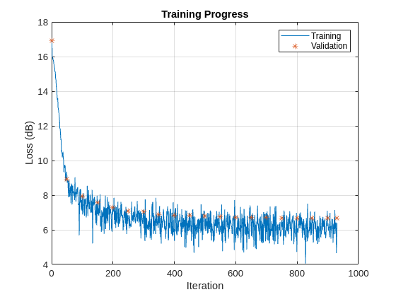
The training and validation loss decreases quickly at first but slows around iteration 400.

Evaluate the Network

Now that the network is trained, view the results for 6 pre-selected evaluation images.

showEvalResultsIdx = [1 3 7 22 25 40];

For each of these evaluation images, plot the original cluttered image, the desired response image, and the network output. The images are all plotted on a log scale with 60 dB of dynamic range.

for idx = showEvalResultsIdx
   helperPlotResult(net2,evalData,evalNormScale,idx)
end

Figure contains 3 axes objects. Axes object 1 with title Original Image contains an object of type image. Axes object 2 with title Ideal Response contains an object of type image. Axes object 3 with title Decluttered Image contains an object of type image.

The network does a decent job of mitigating the unwanted clutter signals while retaining the target signal. The network is able to extrapolate to fill in some of the missing data in cases where the target signal drops out entirely. Some background patches of noise are still present, which might be mitigated by a longer post processing network or additional training.

Conclusion

This example demonstrated how to train and evaluate cascaded convolutional neural networks on PPI and range-time images to remove sea clutter while retaining target returns. It also showed how to define the input and output layers, the hidden convolution, normalization, and activation layers, and configure the training options.

Reference

[1] Vicen-Bueno, Raúl, Rubén Carrasco-Álvarez, Manuel Rosa-Zurera, and José Carlos Nieto-Borge. “Sea Clutter Reduction and Target Enhancement by Neural Networks in a Marine Radar System.” Sensors 9, no. 3 (March 16, 2009): 1913–36.

[2] Zhang, Qi, Yuming Shao, Sai Guo, Lin Sun, and Weidong Chen. “A Novel Method for Sea Clutter Suppression and Target Detection via Deep Convolutional Autoencoder.” International Journal of Signal Processing 2 (2017): 35–40.

Supporting Functions

helperPlotTrainingProgress

function helperPlotTrainingProgress(info)
% Plot training progress

figure
plot(info.TrainingHistory.Iteration,pow2db(info.TrainingHistory.Loss))
hold on
plot(info.ValidationHistory.Iteration,pow2db(info.ValidationHistory.Loss),'*')
hold off
grid on
legend('Training','Validation')
title('Training Progress')
xlabel('Iteration')
ylabel('Loss (dB)')

end

helperPlotEvalResults

function helperPlotEvalResults(imgs,net)
% Plot original images alongside desired and actual responses

for ind = 1:size(imgs,4)
   
    resp_act = predict(net,imgs(:,:,1,ind));
    resp_act(resp_act<0) = 0;
    resp_act = resp_act/max(resp_act(:));
    
    fh = figure;
    
    subplot(1,2,1)
    im = imgs(:,:,1,ind);
    im = im/max(im(:));
    imagesc(mag2db(im))
    clim([-60 0])
    colorbar
    axis equal
    axis tight
    title('Input')
    
    subplot(1,2,2)
    imagesc(mag2db(resp_act))
    clim([-60 0])
    colorbar
    axis equal
    axis tight
    title('Output')
    
    fh.Position = fh.Position + [0 0 560 0];
end

end

helperSegmentData

function [trainIdx,valIdx,testIdx] = helperSegmentData(numSets)

% 80% train, 10% validation, 10% test
props = [0.8 0.1 0.1];

% Training samples
trainIdx = randsample(numSets,floor(props(1)*numSets));

% Get remaining samples
valAndTestIdx = setdiff(1:numSets,trainIdx);

% Validation samples
valIdx = randsample(valAndTestIdx,floor(props(2)*numSets));

% Remaining samples for test
testIdx = setdiff(valAndTestIdx,valIdx);

end

helperPlotResult

function helperPlotResult(net,data,scale,idx)

% Get predicted output using scaled test data input
in = data{1}(:,:,1,idx);
out = predict(net,in);

% Denormalize the input and output for plotting
in = in.*scale(1,:,1,idx);
out = out.*scale(1,:,1,idx);

% It's possible for the network to output negative values for some pixels,
% so we need to take an abs
out = abs(out);

% The ideal response containing only the target image
ideal = data{2}(:,:,1,idx);

% Get color axis limits
mxTgtPwr = mag2db(max(ideal(:)));
cl = [mxTgtPwr-60, mxTgtPwr];

fh = figure;
fh.Position = [fh.Position(1:2) 3*fh.Position(3) fh.Position(4)];

subplot(1,3,1)
imagesc(mag2db(in))
set(gca,'ydir','normal')
colorbar
clim(cl)
title('Original Image')

subplot(1,3,2)
imagesc(mag2db(ideal))
set(gca,'ydir','normal')
colorbar
clim(cl)
title('Ideal Response')

subplot(1,3,3)
imagesc(mag2db(out))
set(gca,'ydir','normal')
colorbar
clim(cl)
title('Decluttered Image')

end