Mission Gap Analysis for Upgrading a Radar System

Define the Mission

Let's improve the primary surveillance radar at an international airport to provide coverage over the entire city and track small targets in this crowded airspace. Right now, there is one primary radar in use by the tracking system at the airport, but it is becoming increasingly apparent that this will not be able to observe all the air traffic over the city and the surrounding mountain ridges and suburbs, called the region of interest (ROI). For this example, you will consider two options to improve the existing system:

Each of these two alternatives will cost the approximately the same amount of money over the operational life cycle of the radar systems. Your objective in this example is to evaluate each of the options to determine the best use of the budget allocated to upgrading the radar system.

Define the Mission Measures

Let's make a version of this for the example:

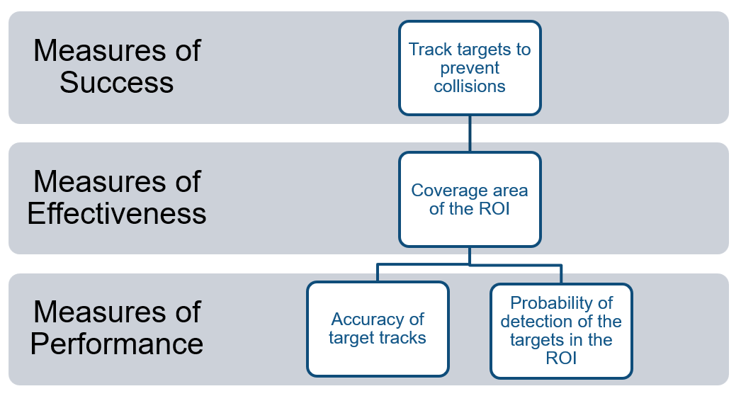
The three measures used in mission-level trade studies are as follows [1]:

For this scenario, define measures for each of these levels for mission success:

% Set random seed for reproducibility
rng default

% Load the region of interest
load("MissionGapAnalysisData.mat","wptsROI")

clear measures
measures.MinAltitude = 1000; % meters above WGS84 ellipsoid
measures.TargetRCS = 1;      % meters-squared
measures.RegionOfInterest = polyshape(wptsROI);
measures.MinCoverage = 0.75;
measures.MaxRMS = 100;       % meters
measures.MinDetect = 0.9;

Analyze Radar Coverage

Baseline Radar

Use helperDesignRadar to load the baseline radar parameters.

% Baseline Radar Location
baselineRdrLat = 40.786444;
baselineRdrLon = -111.978131;

baselineRdrGndHt = helperGroundAltitude(baselineRdrLat,baselineRdrLon);
baselineRdrTwrHt = 10;            % Antenna height (m)
baselineRdrAlt = baselineRdrGndHt + baselineRdrTwrHt;
baselineRdrLLA = [baselineRdrLat, baselineRdrLon, baselineRdrAlt];

% Design the baseline radar system using the output of the Radar Designer
% application
baselineRdrParams = helperDesignRadar("Baseline Radar")

baselineRdrParams=26×2 table
           Parameter              Baseline_Radar   
    ________________________    ___________________

    {'AzimuthBeamwidth'    }    {[  3.0326 3.0326]}
    {'CFARMethod'          }    {["CA"           ]}
    {'CFARNumCells'        }    {[             20]}
    {'ElevationBeamwidth'  }    {[  3.0326 3.0326]}
    {'Frequency'           }    {[     6.0000e+09]}
    {'Gain'                }    {[35.4691 35.4691]}
    {'Height'              }    {[            100]}
    {'MaxSpeed'            }    {[         6.2457]}
    {'NoiseTemperature'    }    {[            290]}
    {'NumCPIs'             }    {[              1]}
    {'NumCoherentPulses'   }    {[              1]}
    {'NumNonCoherentPulses'}    {[              1]}
    {'PRF'                 }    {[            500]}
    {'PeakPower'           }    {[           1800]}
    {'Pfa'                 }    {[     1.0000e-06]}
    {'Polarization'        }    {["H"            ]}
      ⋮

Show the location of the baseline radar and the region of interest where coverage will be measured.

g = geoglobe(uifigure(Name="Scenario"));
hold(g,"on")
hRdr = geoplot3(g,baselineRdrLLA(:,1),baselineRdrLLA(:,2),baselineRdrLLA(:,3),"yo", ...
    LineWidth=6,MarkerSize=1,HeightReference="ellipsoid");
hRoi = geoplot3(g,measures.RegionOfInterest.Vertices(:,1),measures.RegionOfInterest.Vertices(:,2),0,"y", ...
    LineWidth=1,HeightReference="terrain");

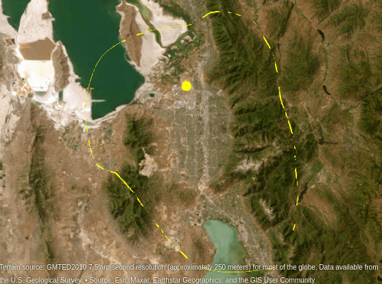
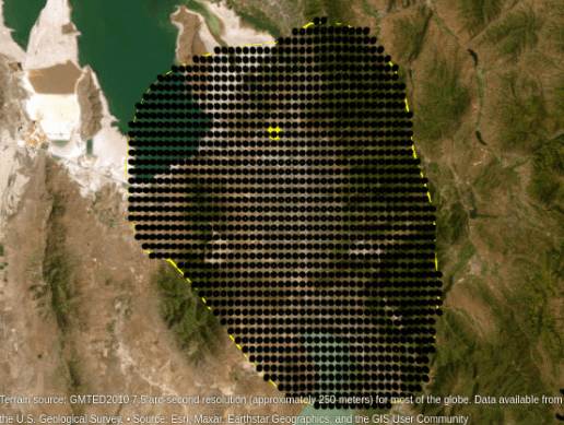
Create a grid of points uniformly distributed across the region of interest. Stack targets at multiple heights at each latitude and longitude to determine the lowest target elevation that can be detected at that location. This grid of points is based on the city, the surrounding suburbs, and typical aircraft routes in the area.

delta = 0.02; % Target spacing in latitude and longitude (degrees)
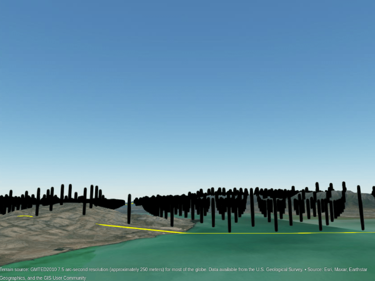
tgtHgtsAGL = 40:20:1000; % Target spacing above ground level (meters)
[tgtLLA,hTgts] = helperRadarCoverageTargetGrid(measures.RegionOfInterest,delta,tgtHgtsAGL,g);
campos(g,40.61,-111.95,120e3);
camheading(g,0); campitch(g,-90); camroll(g,0);

Show how the targets are stacked at multiple heights to search for the lowest detectable target elevation at each latitude and longitude.

campos(g,40.1,-111.9,2.5e3);
camheading(g,10); campitch(g,10); camroll(g,0);

helperRadarCoverageAnalysis computes the signal to noise ratio (SNR) and line of sight visibility for each point in the target grid. The returned, minimum height corresponds to the lowest target elevation for a latitude and longitude with line of sight from the radar to the target and sufficient SNR to be detected by the radar. Use helperRadarCoverageAnalysis to compute the minimum target height for each latitude and longitude location in the target grid.

earth = wgs84Ellipsoid;
scenario = setupScenario(tgtLLA);

baselineRdrMinHts = helperRadarCoverageAnalysis(baselineRdrParams, baselineRdrLLA, tgtLLA, measures, scenario, earth);

Plot the radar coverage over the target grid. The target grid location colors are assigned according to the lowest detectable target height. The black region represents the area where targets cannot be detected with the required probability of detection.

hDets = plotRadarCoverage(baselineRdrMinHts,tgtLLA,g);
campos(g,40.61,-111.95,120e3);
camheading(g,0); campitch(g,-90); camroll(g,0);

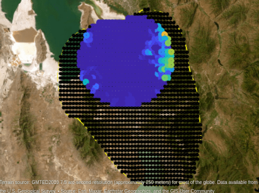
Calculate the fraction of the region of interest covered by the baseline radar. The objective based on our MOE as stated above is to maximize this fraction.

radarCoverageFraction(baselineRdrMinHts)

Percent area coverage:
    0.3557

The gap in the baseline radar's coverage is evident. The baseline radar's coverage is well below the 75% established as a measure of effectiveness for this mission.

Enhanced Radar

Use helperDesignRadar to load in the design parameters for the enhanced radar. Compute the coverage for the enhanced radar. For this option, the enhanced radar increases the peak power and number of coherently integrated pulses for the existing radar to improve its maximum detection range.

enhancedRdrParams = helperDesignRadar("Enhanced Radar")

enhancedRdrParams=26×2 table
           Parameter              Enhanced_Radar   
    ________________________    ___________________

    {'AzimuthBeamwidth'    }    {[  3.0326 3.0326]}
    {'CFARMethod'          }    {["CA"           ]}
    {'CFARNumCells'        }    {[             20]}
    {'ElevationBeamwidth'  }    {[  3.0326 3.0326]}
    {'Frequency'           }    {[     6.0000e+09]}
    {'Gain'                }    {[35.4691 35.4691]}
    {'Height'              }    {[            100]}
    {'MaxSpeed'            }    {[         6.2457]}
    {'NoiseTemperature'    }    {[            290]}
    {'NumCPIs'             }    {[              1]}
    {'NumCoherentPulses'   }    {[              1]}
    {'NumNonCoherentPulses'}    {[             10]}
    {'PRF'                 }    {[            500]}
    {'PeakPower'           }    {[           3600]}
    {'Pfa'                 }    {[     1.0000e-06]}
    {'Polarization'        }    {["H"            ]}
      ⋮

enhancedRdrLLA = baselineRdrLLA;

enhancedRdrMinHts = helperRadarCoverageAnalysis(enhancedRdrParams, enhancedRdrLLA, tgtLLA, measures, scenario, earth);

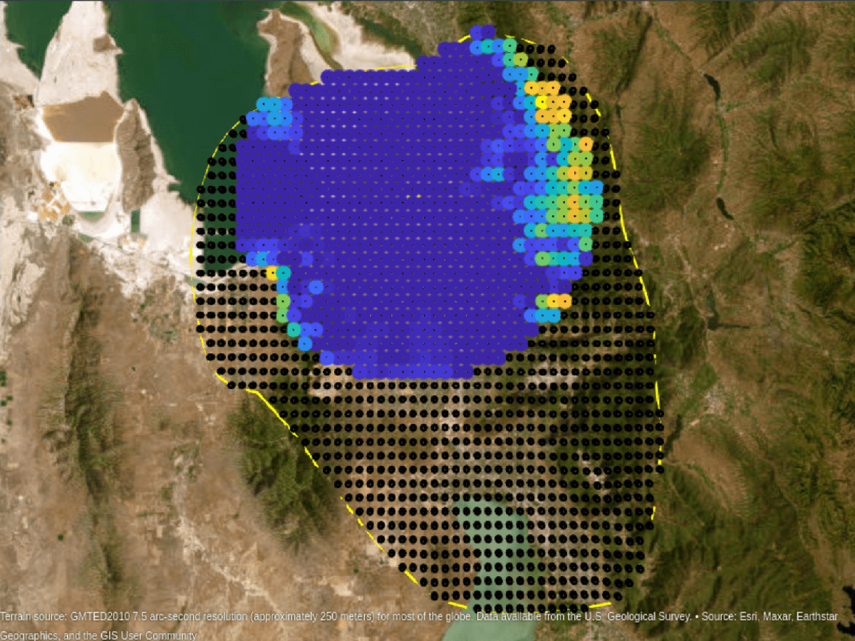
Show the coverage for the enhanced radar.

delete(hDets(ishghandle(hDets)));
hDets = plotRadarCoverage(enhancedRdrMinHts,tgtLLA,g);

radarCoverageFraction(enhancedRdrMinHts)

Percent area coverage:
    0.4672

The enhanced radar increases the coverage area over the baseline radar, but a large portion of the region to the south remains undetected by the radar.

Multiple Radars

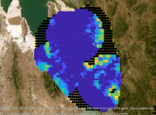
The multiple radar option repeats the same baseline radar configuration at two additional sites. These sites were chosen because of their ideal placement on top of ridges in strategic positions in the ROI without previously existing buildings. See the Planning Radar Network Coverage over Terrain example for details on how to select locations to optimize radar coverage.

Compute the radar coverage for the multiple radar option.

multRdrLat = [baselineRdrLat - 0.2735, baselineRdrLat - 0.371];
multRdrLon = [baselineRdrLon - 0.209, baselineRdrLon + 0.3105];

multRdrAlt = helperGroundAltitude(multRdrLat,multRdrLon) + 20;
multRdrLLA = [baselineRdrLLA; multRdrLat(:) multRdrLon(:) multRdrAlt(:)];

multiRdrParams = helperDesignRadar("Multiple Radars");

hMultRdr = geoplot3(g,multRdrLLA(2:end,1),multRdrLLA(2:end,2),multRdrLLA(2:end,3),"go", ...
    LineWidth=6,MarkerSize=1,HeightReference="ellipsoid");

multRdrMinHts = helperRadarCoverageAnalysis(multiRdrParams, multRdrLLA, tgtLLA, measures, scenario, earth);

delete(hDets(ishghandle(hDets)));
hDets = plotRadarCoverage(multRdrMinHts,tgtLLA,g);

radarCoverageFraction(multRdrMinHts)

Percent area coverage:
    0.7956

The multiple radar option achieves the 75% measure of effectiveness required for this mission but covers less of the mountain ridge near the airport than the enhanced radar.

Analyze Radar Tracks

The coverage analysis in the preceding section shows that the multiple radar option satisfies the measure of effectiveness for the mission, but the mission measure of performance requires analysis of the radar tracks.

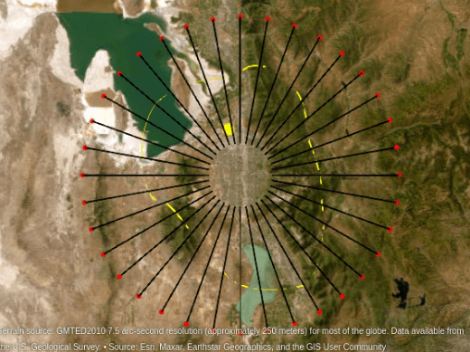
Create a scenario with inbound targets spaced every 10 degrees at the center of the region of interest. Use track metrics for each of these targets to compute the percent of time the targets are tracked inside the region of interest and the range where the RMS position accuracy is achieved.

[lat0, lon0] = centroid(measures.RegionOfInterest);
alt0 = helperGroundAltitude(lat0,lon0);
lla0 = [lat0 lon0 alt0];

% Define end point for target trajectories
endLLA = [lat0 lon0 measures.MinAltitude].';

% Define starting points for target trajectories
tgtAz = 0:10:359;
tgtRg = 65e3;
[tgtNorth,tgtEast] = pol2cart(-deg2rad(tgtAz),tgtRg);
[tgtLat,tgtLon] = enu2geodetic(tgtEast(:),tgtNorth(:),zeros(numel(tgtEast),1),endLLA(1),endLLA(2),endLLA(3),earth);
startLLA = [tgtLat(:) tgtLon(:) measures.MinAltitude*ones(numel(tgtAz),1)].';

scenario = setupScenario([startLLA endLLA]);
plat = platform(scenario,Position=baselineRdrLLA);

Use helperDesignRadar to configure the baseline radarDataGenerator sensor model. The radarDataGenerator is a measurement level model of the radar system that uses probability of detection, probability of false alarm, and information about noise and biases in the scenario and radar system to generate tracks representative of what the radar systems under test would produce.

baselineRadar = helperDesignRadar(baselineRdrParams);

To simplify the simulation, set the azimuth field of view for the radar to 360 degrees to model a radar that reports tracks at the completion of each 360-degree scan. This avoids the need to collect track metrics at all intermediate scan positions.

baselineRadar.ScanMode = "No scanning";
baselineRadar.FieldOfView(1) = 360;

Set the radar to report tracks in the scenario frame. Ensure the INS input on the radar is enabled so that the detections can be transformed into the scenario frame by the tracker.

baselineRadar.HasINS = true;
baselineRadar.TargetReportFormat = "Tracks";
baselineRadar.TrackCoordinates = "Scenario";

Disable false alarm reporting to simplify the collection and analysis of the track metrics.

baselineRadar.HasFalseAlarms = false;

Attach the baseline radar to the radar platform in the scenario.

plat.Sensors = baselineRadar;

Specify the speed and minimum height above the ground for the targets. Use helperRadarTrackTargets to generate the trajectories from the starting and ending waypoints for the radially inbound targets.

kts2mps = unitsratio("m","km")/3600;
tgtSpd = 300*kts2mps;
minHtAGL = 500;

wpts = helperRadarTrackTargets(scenario,tgtSpd,minHtAGL,startLLA,endLLA,measures,earth);

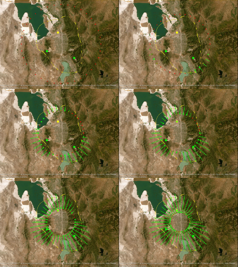
Visualize the target trajectories. The targets are the red circles on the map and the black lines are the trajectories the targets will follow as they move into the region of interest.

delete(hTgts(ishghandle(hTgts)));
delete(hMultRdr(ishghandle(hMultRdr)));
delete(hDets(ishghandle(hDets)));

tgts = scenario.Platforms(2:end);
numTgts = numel(tgts);
tgtLLA = NaN(numTgts,3);
for iTgt = 1:numTgts
    thisTgt = tgts{iTgt};
    tgtLLA(iTgt,:) = thisTgt.Trajectory.Waypoints(1,:);
end

hTgts = NaN(1,2);
hTgts(1) = geoplot3(g,tgtLLA(:,1),tgtLLA(:,2),tgtLLA(:,3),"ro", ...
    MarkerSize=0.5,LineWidth=2,HeightReference="ellipsoid");
hTgts(2) = geoplot3(g,wpts(1,:),wpts(2,:),wpts(3,:),"k-", ...
    LineWidth=1,HeightReference="ellipsoid");
camheight(g,170e3);

Baseline Radar

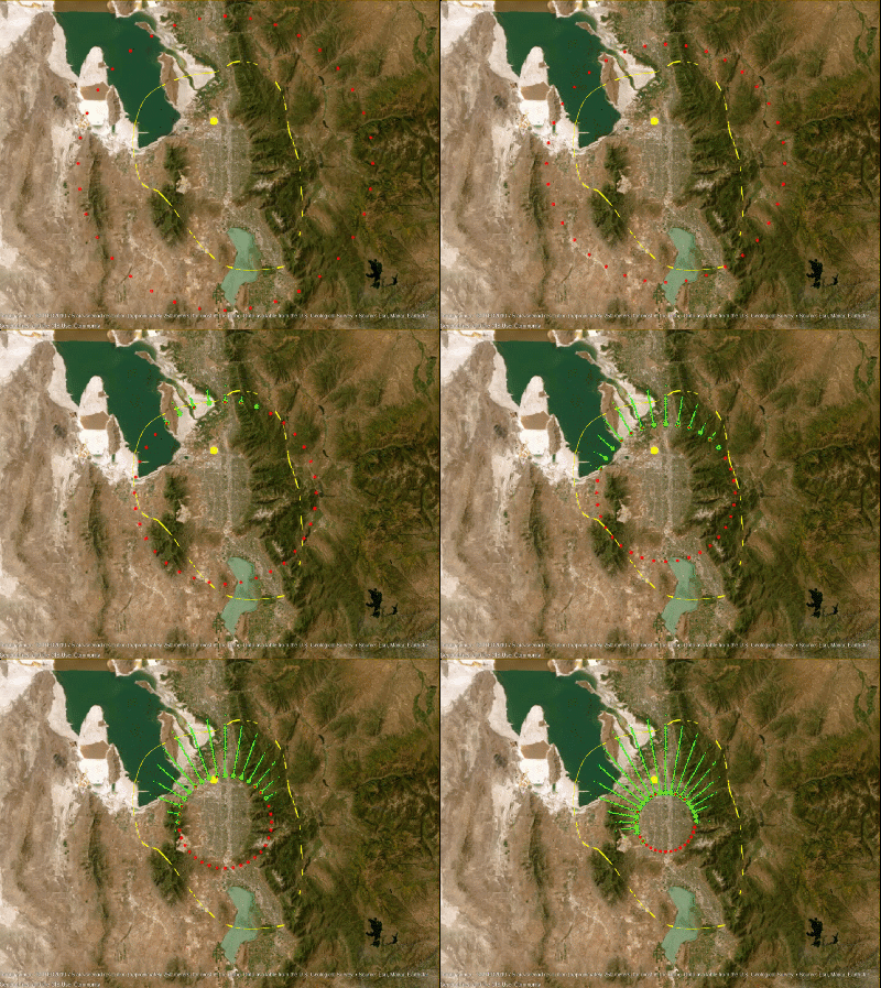
Use helperRadarTrackAnalysis to run the simulation and collect the track metrics. During the simulation, you will see the red targets moving radially inward towards the center of the region of interest. The target tracks are shown in green.

[baselineMetrics,hTgts] = helperRadarTrackAnalysis(scenario, earth, g, hTgts);

Plot the overall probability of detection and positional track RMS accuracy as a function of their range from the center of the region of interest.

tl = tiledlayout(figure,2,1);
set(helperPlotTrackMetrics(tl,baselineMetrics,measures,lla0,earth),"DisplayName","Baseline");

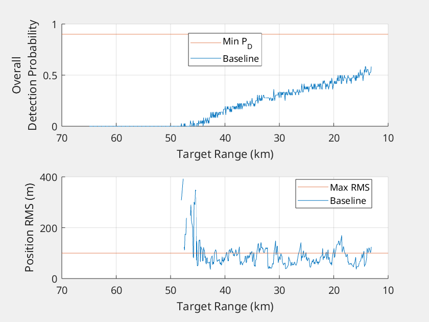
The plot on the top shows the overall detection probability observed in the simulation across all inbound targets. The plot on the bottom shows the overall position RMS across all targets. The baseline radar is unable to meet either of these measures of performance for this mission.

Enhanced Radar

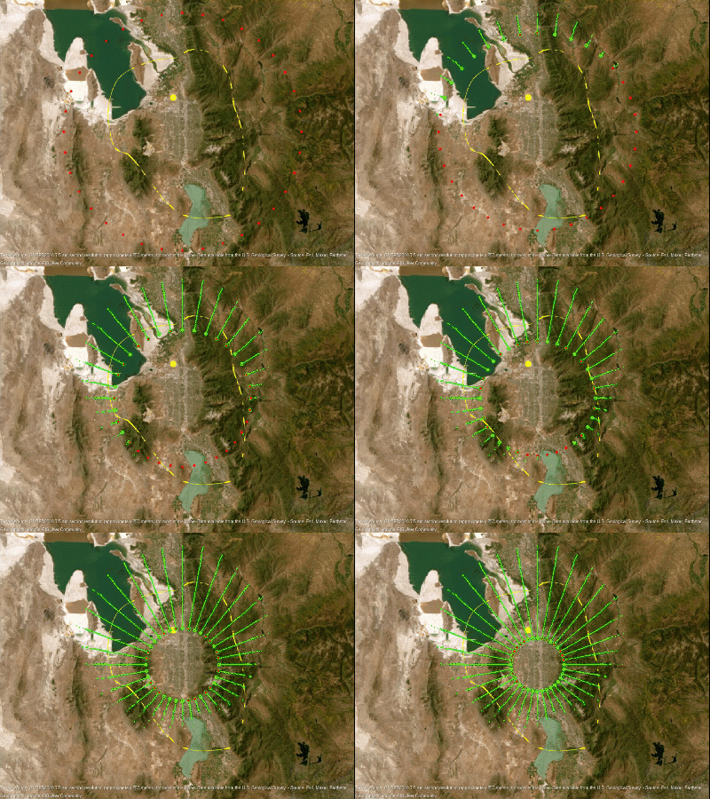
Use helperDesignRadar to configure the radarDataGenerator sensor model for the enhanced radar and reproduce the track analysis.

enhancedRadar = helperDesignRadar(enhancedRdrParams);

enhancedRadar.SensorIndex = 2;
enhancedRadar.ScanMode = "No scanning";
enhancedRadar.FieldOfView(1) = 360;
enhancedRadar.HasINS = true;
enhancedRadar.TargetReportFormat = "Tracks";
enhancedRadar.TrackCoordinates = "Scenario";
enhancedRadar.HasFalseAlarms = false;

plat.Sensors = enhancedRadar;

[enhancedMetrics,hTgts] = helperRadarTrackAnalysis(scenario, earth, g, hTgts);

set(helperPlotTrackMetrics(tl,enhancedMetrics,measures,lla0,earth),"DisplayName","Enhanced");

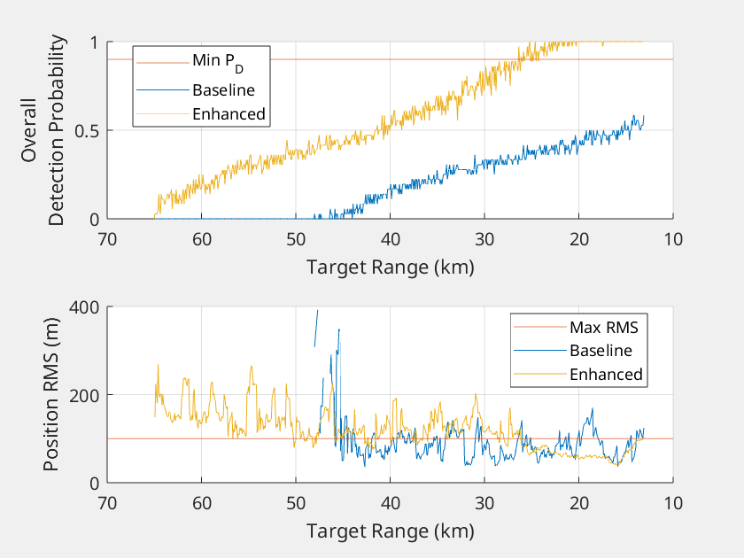
As already seen in the radar coverage analysis, the enhanced radar provides higher detection probabilities at ranges much farther from the center of the region of interest. The overall track quality is much better as well, with the overall position RMS error staying below the 100 m requirement at around 25 km.

Multiple Radars

Finally, apply the same simulation and track analysis to the second radar improvement option which places two identical radars in the region of interest to provide detections to a central tracker in addition to the detections reported by the existing baseline radar.

% Add additional radar sites to globe viewer
delete(hMultRdr(ishghandle(hMultRdr)));
hMultRdr = geoplot3(g,multRdrLLA(2:end,1),multRdrLLA(2:end,2),multRdrLLA(2:end,3),"go", ...
    LineWidth=6,MarkerSize=1,HeightReference="ellipsoid");

% Create scenario with multiple radar sites
scenario = setupScenario([startLLA endLLA]);

radar = clone(baselineRadar);
release(radar);
radar.TargetReportFormat = "Clustered detections";
radar.DetectionCoordinates = "Sensor spherical";
for iPlat = 1:size(multRdrLLA,1)
    plat = platform(scenario,Position=multRdrLLA(iPlat,:));
    thisRadar = clone(radar);
    thisRadar.SensorIndex = iPlat;
    plat.Sensors = thisRadar;
end

helperRadarTrackTargets(scenario,tgtSpd,minHtAGL,startLLA,endLLA,measures,earth);

[multMetrics,hTgts] = helperRadarTrackAnalysis(scenario, earth, g, hTgts);

set(helperPlotTrackMetrics(tl,multMetrics,measures,lla0,earth),"DisplayName","Multiple");

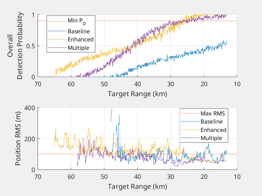
Multiple radar locations demonstrate better overall detection performance than the enhanced radar at about 40 km. Both options attain the required detection probability at approximately 25 km. The positional RMS errors are maintained below the 100 m threshold at much longer ranges than with the enhanced radar.

Conclusion

In this example, you evaluated two proposed improvements for an existing radar system to satisfy a new mission objective. One option was to improve the existing radar to improve its maximum detection range. The other option was to add two additional radar sites that are operationally equivalent to the existing radar, with all three radars sharing their detections with a central tracker.

These two options will cost the same amount of money but led to different outcomes as demonstrated by the analysis. The first alternative architecture, an enhanced radar, was an improvement over the baseline and enabled more coverage of the area of interest. The enhanced radar enabled coverage of 47% of the region of interest. Both the enhanced and multiple radar options attained the required overall detection probability of 90% at approximately 25 km. However, the multiple radar option satisfied the coverage requirement for the region of interest with approximately 80% coverage. The multiple radar option also achieved a lower RMS track position error than the enhanced radar option, especially at longer ranges from the center of the region of interest.

The conclusion from this analysis is to invest in installing two new radar site locations at strategic positions on the ridges neighboring the city.

Reference

[1] Office of the Under Secretary of Defense for Research and Engineering. Department of Defense Mission Engineering Guide (MEG) version 2.0. 1 Oct. 2023, https://ac.cto.mil/wp-content/uploads/2023/11/MEG_2_Oct2023.pdf.

Helper Functions

function scenario = setupScenario(wptsLLA)
% Returns scenario with land surface added with terrain covering the full
% region defined in wptsLLA

if isstruct(wptsLLA)
    latLim = [inf, -inf];
    lonLim = [inf, -inf];
    for ii = 1:numel(wptsLLA)
        lla = wptsLLA(ii).LLA;

        [latMin, latMax] = bounds(lla(1,:));
        [lonMin, lonMax] = bounds(lla(2,:));

        latLim(1) = min(latMin, latLim(1));
        latLim(2) = max(latMax, latLim(2));

        lonLim(1) = min(lonMin, lonLim(1));
        lonLim(2) = max(lonMax, lonLim(2));
    end
else
    [latMin, latMax] = bounds(wptsLLA(1,:));
    [lonMin, lonMax] = bounds(wptsLLA(2,:));
    latLim = [latMin latMax];
    lonLim = [lonMin lonMax];
end

scenario = radarScenario(UpdateRate=0,IsEarthCentered=true);

% Load digital elevation map to model terrain
layers = wmsfind("mathworks","SearchField","serverurl");
elevation = refine(layers,"elevation");

[A,R] = wmsread(elevation,Latlim=latLim,Lonlim=lonLim, ...
    ImageFormat="image/bil");

% The elevation map contains orthometric heights referenced to the EGM96
% geoid. Use egm96geoid to convert these heights to ellipsoidal heights
% referenced to the WGS84 ellipsoid.

% Reference heights to the WGS84 ellipsoid
N = egm96geoid(R);
Z = double(A) + N;

landSurface(scenario,Terrain=flipud(Z).', ...
    Boundary=[R.LatitudeLimits;R.LongitudeLimits]);
end

function h = plotRadarCoverage(minHt,tgtLLA,g)
% Plots the radar coverage showing the minimum height targets can be
% detected at in the geoglobe, g. Returns the graphics handle to the
% plotted coverage map.

numTgtHts = size(tgtLLA,3);

clrs = parula(numTgtHts);
h = NaN(1,numTgtHts);
for iHt = 1:numTgtHts
    thisClr = clrs(iHt,:);
    isThis = minHt==iHt;

    if any(isThis)
        theseTgts = tgtLLA(:,:,iHt);
        h(iHt) = geoplot3(g,theseTgts(1,isThis),theseTgts(2,isThis),theseTgts(3,isThis)+ 1000,"o", ...
            Color=thisClr,LineWidth=6,MarkerSize=1,HeightReference="ellipsoid");
    end
end
end

function radarCoverageFraction(minHt)
% Returns the fraction of the area where targets are detectable
numTot = numel(minHt);
numDet = sum(isfinite(minHt(:)));
disp("Percent area coverage:")
disp(numDet/numTot)
end