Modeling the Propagation of Radar Signals

Introduction

To properly evaluate the performance of radar and wireless communication systems, it is critical to understand the propagation environment. The received signal power of a monostatic radar is given by the radar range equation:

where is the transmitted power, is the antenna gain, is the target radar cross section (RCS), is the wavelength, and is the propagation distance. All propagation losses other than free space path loss are included in the term. The rest of the example shows how to estimate this term in different scenarios.

Free Space Path Loss

Free space path loss is computed as a function of propagation distance and frequency. In free space, RF signals propagate at the speed of light in all directions. At a far enough distance, the radiating source looks like a point in space and the wavefront forms a sphere whose radius is equal to . The power density at the wavefront is inversely proportional to :

where is the transmitted signal power. For a monostatic radar where the signal has to travel both directions (from the source to the target and back), the dependency is actually inversely proportional to , as shown previously in the radar equation. The loss related to this propagation mechanism is referred to as free space path loss, sometimes also called the spreading loss. Quantitatively, free space path loss is also a function of frequency, given by [5]:

As a convention, propagation losses are often expressed in dB. This convention makes it much easier to derive the two-way free space path loss by simply doubling the one-way free space loss.

Use the fspl function to calculate the free-space path loss, and plot the loss for frequencies between 1 and 1000 GHz, for different ranges.

c = physconst('lightspeed');
R0 = [100 1e3 10e3];
freq = (1:1000).'*1e9;
apathloss = fspl(R0,c./freq);
loglog(freq/1e9,apathloss);
grid on;
ylim([90 200]);
legend('Range: 100 m', 'Range: 1 km', 'Range: 10 km','Location','northwest');
xlabel('Frequency (GHz)');
ylabel('Path Loss (dB)');
title('Free Space Path Loss');

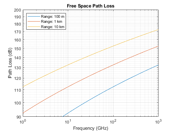
The figure shows that the propagation loss increases with range and frequency.

Propagation Loss Due to Precipitation and Atmosphere

In reality, signals do not always travel in a vacuum, so free space path loss describes only part of the signal attenuation. Signals interact with particles in the air and lose energy along the propagation path. The loss varies with different factors such as pressure, temperature, and water density.

Loss Due to Rain and Snow

Rain can be a major limiting factor for radar systems, especially when operating above 5 GHz. In the ITU model in [2], rain is characterized by the rain rate (in mm/h). According to [6], the rain rate can range from less than 0.25 mm/h for very light rain to over 50 mm/h for extreme rains. In addition, because of the rain drop's shape and its relative size compared to the RF signal wavelength, the propagation loss due to rain is also a function of signal polarization. In general, horizontal polarization represents the worst case for propagation loss due to rain.

The functions rainpl and cranerainpl can be used to compute losses due to rain according to the ITU and Crane models, respectively. Both models are valid between 1 GHz and 1 THz. Let the polarization be horizontal, so the tilt angle is 0, and let the signal propagate parallel to the ground, so the elevation angle is 0. Plot losses computed with both models and compare.

R0 = 5e3;                % 5 km range
rainrate = [1 4 20];     % rain rate in mm/h
el = 0;                  % 0 degree elevation
tau = 0;                 % horizontal polarization

for m = 1:numel(rainrate)
    rainloss_itu(:,m) = rainpl(R0,freq,rainrate(m),el,tau)';
    rainloss_crane(:,m) = cranerainpl(R0,freq,rainrate(m),el,tau)';
end
loglog(freq/1e9,rainloss_itu);
hold on;
set(gca,'ColorOrderIndex',1); % reset color index for better comparison
loglog(freq/1e9,rainloss_crane,'--');
hold off;
grid on;
legend('Light Rain (ITU)','Moderate Rain (ITU)','Heavy Rain (ITU)',...
    'Light Rain (Crane)','Moderate Rain (Crane)','Heavy Rain (Crane)', ...
    'Location','SouthEast');
xlabel('Frequency (GHz)');
ylabel('Attenuation at 5 km (dB)')
title('Rain Attenuation for Horizontal Polarization');

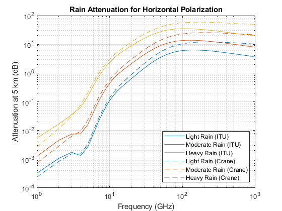
The losses computed with the Crane model are mostly larger than the losses computed with the ITU model at this propagation range. At smaller propagation ranges and lower frequencies, the ITU model may output a smaller attenuation value than Crane. Note that the models differ greatly enough that at higher frequencies, light rainfall for one model may have the same attenuation as moderate rainfall for the other model.

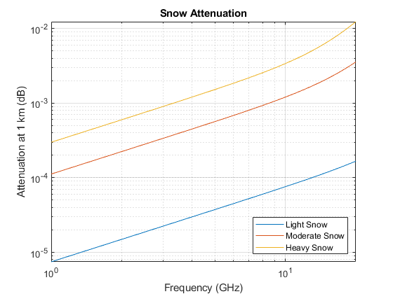
Similar to rainfall, snow can also have a significant impact on the propagation of RF signals. A common practice is to treat snow as rainfall and compute the propagation loss based on the rain model, even though this approach tends to overestimate the loss a bit. Attenuation due to propagation through snow is not considered dependent on polarization, but is highly dependent on frequency. The model for losses due to snow is parameterized by the equivalent liquid content instead of volume. For a given water content, snow requires about 10 times as much volume as rain.

Use the snowpl function to compute losses due to snow, and plot the losses against frequency. By default, this function uses the Gunn-East attenuation model, which is generally valid up to about 20 GHz.

freq = (1:20)*1e9;
R0 = 1e3;               % 1 km range
snowrate = [0.1 1.5 4]; % equivalent liquid water content in mm/h

for m = 1:numel(snowrate)
    snowloss(:,m) = snowpl(R0,freq,snowrate(m));
end
loglog(freq/1e9,snowloss);
grid on;
legend('Light Snow','Moderate Snow','Heavy Snow', ...
    'Location','SouthEast');
xlabel('Frequency (GHz)');
ylabel('Attenuation at 1 km (dB)')
title('Snow Attenuation');

Loss Due to Fog and Cloud

Fog and cloud are formed with water droplets too, although much smaller compared to rain drops. The size of fog droplets is generally less than 0.01 cm. Fog is often characterized by the liquid water density. A medium fog with a visibility of roughly 300 meters, has a liquid water density of 0.05 g/m^3. For heavy fog where the visibility drops to 50 meters, the liquid water density is about 0.5 g/m^3. The atmosphere temperature (in Celsius) is also present in the ITU model for propagation loss due to fog and cloud [3].

Use the fogpl function to compute losses due to fog, and plot the losses against frequency. The ITU model for attenuation due to fog is valid between 10 GHz and 1 THz.

freq = (10:1000)*1e9;
T = 15;                         % 15 degree Celsius
waterdensity = [0.01 0.05 0.5]; % liquid water density in g/m^3
for m = 1: numel(waterdensity)
    fogloss(:,m) = fogpl(R0,freq,T,waterdensity(m))';
end
loglog(freq/1e9,fogloss);
grid on;
legend('Light Fog','Medium Fog','Heavy Fog','Location','southeast');
xlabel('Frequency (GHz)');
ylabel('Attenuation at 1 km (dB)')
title('Fog Attenuation');

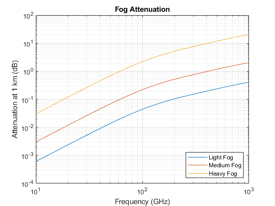
Note that in general fog is not present when it is raining.

Loss Due to Atmospheric Absorption and Lensing

Even when there is no fog or rain, the atmosphere is full of gases that still affect the signal propagation. The ITU model [4] describes atmospheric gas attenuation as a function of both dry air pressure, like oxygen, measured in hPa, and water vapour density, measured in g/m^3.

Use the tropopl function to compute losses due to atmospheric absorption, and plot the losses against frequency. By default, this function uses the Mean Annual Global Reference Atmosphere (MAGRA) model to get typical values of temperature, pressure, and water vapor density for a given altitude. We can also specify a latitude model to use a model tailored for a specific range of latitudes. Some latitude models also allow for specification of a season. Let our altitude be 2 km (note that the troposphere, for which this model is valid, extends up to 10 km) and our propagation path be depressed by 5 degrees. This function returns the total loss due to atmospheric absorption over the slanted propagation path, but does not include dissipation due to refraction (lensing). Compare losses between the low, mid, and high latitude models.

height = 2e3;
el = -5; % elevation angle
atmloss_low = tropopl(R0,freq,height,el,'LatitudeModel','Low');
atmloss_mid = tropopl(R0,freq,height,el,'LatitudeModel','Mid');
atmloss_high = tropopl(R0,freq,height,el,'LatitudeModel','High');
loglog(freq/1e9,atmloss_low);
hold on;
loglog(freq/1e9,atmloss_mid);
loglog(freq/1e9,atmloss_high);
hold off;
grid on;
legend('Low Latitudes','Mid Latitudes','High Latitudes','Location','northwest');
xlabel('Frequency (GHz)');
ylabel('Attenuation at 1 km (dB)')
title('Atmospheric Gas Attenuation');

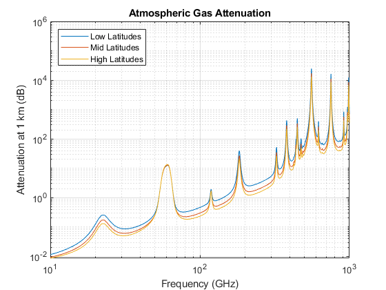
The plot suggests that there is a strong absorption due to atmospheric gases at around 60 GHz.

Another source of losses due to atmosphere is from atmospheric lensing. This is a phenomenon whereby the angular extent of a transmission is increased with range due to a refractivity gradient. This spreading of energy decreases the energy density along the nominal (straight) propagation path, independent of frequency.

Atmospheric pressure, and thus refractivity, changes with altitude. So for a given height, the elevation angle of the propagation path is enough to determine losses due to this effect.

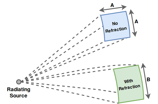
Use the lenspl function to compute these losses and plot against frequency. Because this loss is independent of frequency, plot the loss against propagation range for a set of heights. Use an elevation angle of 0.05 degrees for a slanted propagation path.

R = 1e3:1e3:100e3;      % propagation range
el = 0.05;              % elevation angle
heights = [10 100 200]; % radar platform heights
for m = 1:numel(heights)
    lenloss(:,m) = lenspl(R,heights(m),el);
end
semilogy(R/1e3,lenloss);
grid on;
legend('Height: 10 m','Height: 100 m','Height: 200 m','Location',...
    'southeast');
xlabel('Propagation Range (km)');
ylabel('Attenuation (dB)')
title('Atmospheric Lensing Attenuation');

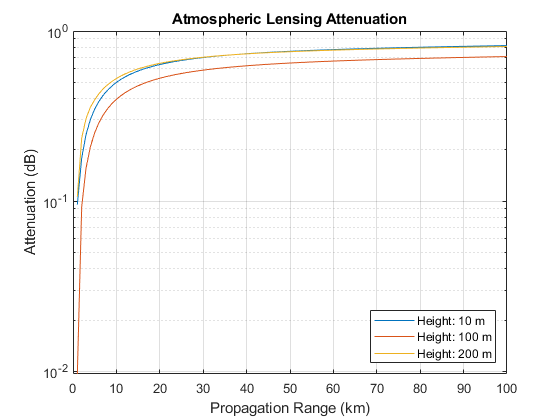
Attenuation due to lensing decreases as altitude increases. For convenience, attenuation due to lensing is also provided as a secondary output from tropopl.

Loss Due to Polarization Mismatch

Some types of propagation loss are dependent on the polarization of the transmitted radiation, such as with rain loss. This is a result of the chemical and structural properties of the medium. However, even in free space there may be losses due to a mismatch of the propagated polarization vector and the polarization of the receiving antenna. For example, if the propagated polarization vector is orthogonal to the polarization of the receiving antenna, almost no direct signal energy would be received. Note that the propagated polarization vector is not in general the same as the transmitted polarization vector, as the direction of propagation must be taken into account. Note also that the other loss functions which take polarization as an input do not compute losses due to this mismatch. Polarization-dependent losses due to properties of the propagation medium can be handled separately from losses due to polarization mismatch, as the latter is heavily dependent on the transmitter/receiver orientation.

Use the polloss function to compute the loss due to polarization mismatch for a given transmit/receive polarization, platform positions, and platform orientations. Place the transmit platform at the origin with no rotation from inertial. Place the receive platform along the X axis and compute polarization loss for a range of roll angles. Let the antenna polarizations both be vertical.

poltx = [0;1];  % [H;V] polarization
polrx = [0;1];
postx = [0;0;0];
posrx = [100;0;0];
frmtx = eye(3); % transmit frame aligned with inertial
rolls = 0:180;

for m = 1:numel(rolls)
    frm_r = rotx(rolls(m));
    rho(m) = polloss(poltx,polrx,posrx,frm_r,postx,frmtx);
end

semilogy(rolls,rho);
grid on;
xlabel('Roll Angle (deg)');
ylabel('Attenuation (dB)');
title('Attenuation Due to Polarization Mismatch');

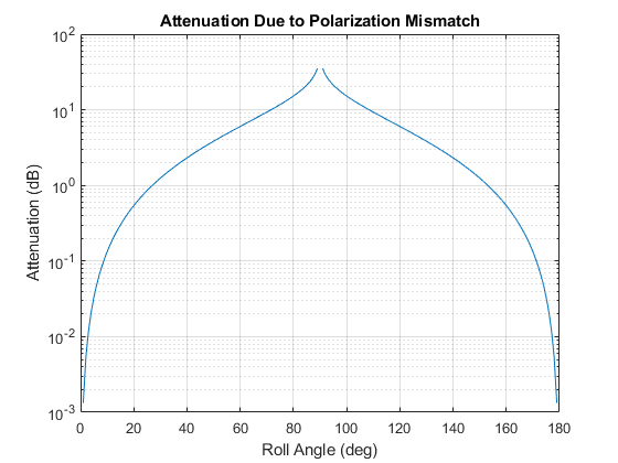
The attenuation approaches infinity at a 90 degree roll angle.

Radar Propagation Factor and Vertical Coverage Diagram

When transmitting over a wide angle or from an antenna close to the ground, multipath from ground bounce, along with refraction from atmosphere, yields a radiation pattern at a given range that can be quite different from the nominal transmit pattern. This is captured by the radar propagation factor, which is the ratio of the actual field strength relative to what the field strength would be in free space. The propagation factor can vary greatly as the relative phase between the direct and indirect path signals changes.

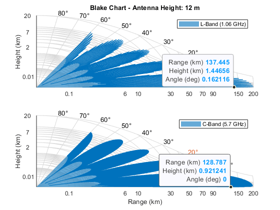
A vertical coverage diagram (Blake chart) is a compact way of displaying contours of fixed signal energy (such as a minimum signal power for detection) as a function of propagation range and elevation angle. Only the vertical plane in which both the direct and indirect path signals propagate is considered.

The function radarvcd takes a reference range as input and returns the range at which the received power in the multipath environment equals what it would be in free space. This effective range is plotted on a range-height-angle chart. This can quickly give, for example, the actual detection range given a free-space detection range, as a function of range, height, or elevation angle.

Use a free-space detection range of 100 km, transmit frequencies in L-Band and C-Band, and an antenna height of 12 m. A sinc transmit pattern is used by default.

freq = [1.06 5.7]*1e9; % L-Band and C-Band transmit frequencies (Hz)
antht = 12;            % height of antenna (m)
rngfs = 100;           % free-space detection range (km)
for m = 1:numel(freq)
    [vcp{m}, vcpang{m}] = radarvcd(freq(m),rngfs,antht);
end

blakechart takes these detection ranges and angles, along with additional atmospheric properties to create the Blake chart. Use the refractiveidx function to compute the corresponding refraction exponent for input to blakechart.

[~,N] = refractiveidx(0); % atmospheric refractivity at the surface
helperPlotBlakeChart(vcp,vcpang,N)

Ground-bounce interference dominates the propagation factor for shorter ranges, in the so-called interference region, but at longer ranges and low elevation angles the propagation factor is dominated by diffraction over the horizon, the diffraction region. Use the radarpropfactor function to compute the propagation factor for an interval of ranges and observe the difference between these two regions.

Compute the propagation factor for a fixed height above the surface of 1 km and propagation ranges between 50 and 200 km. Set the surface slope and height standard deviation to 0 to represent a smooth surface. Perform the analysis for the two frequency bands.

tgtht = 1e3;           % target height (m)
R = (50:200)*1e3;      % propagation range (m)
Re = effearthradius;   % effective Earth radius (m)
Rd = sqrt(2*Re)*(sqrt(antht) + sqrt(tgtht)); % diffraction range
F = zeros(numel(freq),numel(R));
for m = 1:numel(freq)
    F(m,:) = radarpropfactor(R,freq(m),antht,tgtht,'SurfaceHeightStandardDeviation',0,'SurfaceSlope',0);
end
helperPlotPropagationFactor(R,F,Rd)

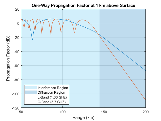
The propagation factor oscillates in the interference region, then decreases quickly in the diffraction region.

Combine the ground-bounce interference and atmospheric absorption losses. Assume in this calculation that a 3.3 GHz S-band surface ship radar is 20 m above the water and has an elevation beamwidth of 30 deg.

freq = 3.3e9;                   % Frequency (Hz)
elbw = 30;                      % Elevation beamwidth (deg)
Rkm = 1:0.1:120;                % Range (km)
R = Rkm.*1e3;                   % Range (m)
[htsd,beta0] = searoughness(1); % Sea surface
anht = 20 + 2*htsd;             % Radar height (m)
tgtht = (anht+1):1:300;         % Target height (m)

% Calculate combined environment losses for different heights and ranges
[PLdB, PLdBNorm] = helperCombineEnvLosses(R,freq,anht,tgtht,htsd,beta0,elbw);

% Plot combined losses for different heights and ranges
helperPlotCombinedEnvLosses(Rkm,freq,anht,tgtht,PLdBNorm)

Multipath Propagation, Time Delays, and Doppler Shifts

Signals may not always propagate along the line of sight, but arrive at the destination via different paths and may add up either constructively or destructively. This multipath effect can cause significant fluctuations in the received signal power.

The functions mentioned in the previous sections for computing propagation losses are useful to establish budget links, but to simulate the propagation of arbitrary signals, you also need to apply range-dependent time delays, gains, and phase shifts. Various channel objects are available to model multipath propagation. For a simple line-of-sight path, use the phased.LOSChannel object to model the propagation subject to any of the loss types described previously.

Ground reflection is a common phenomenon for many radar or wireless communication systems. For example, when a ground-based or sea-based radar illuminates a target, the signal not only propagates along the direct line of sight but is also reflected from the ground. Use the twoRayChannel object to model the combination of a direct path and single-bounce path, such as for ground reflection.

Time Delays and Doppler Shifts

First, define the transmitted signal. Use a rectangular waveform.

waveform = phased.RectangularWaveform('PRF',250);
wav = waveform();

Assume an L-band operating frequency of 1.9 GHz. Model the channel.

fc = 1.9e9;
channel = twoRayChannel('PropagationSpeed',c,'OperatingFrequency',fc);

Assume the target unit is 1.65 km above the ground, the radar antenna is 12 meters above the ground at a 50 km distance. Simulate the signal as it reaches the target.

pos_radar = [0;0;12];
pos_target = [50e3;0;1.65e3];
vel_radar = [0;0;0];
vel_target = [-200;0;0];
y2ray = channel(wav,pos_radar,pos_target,vel_radar,vel_target);

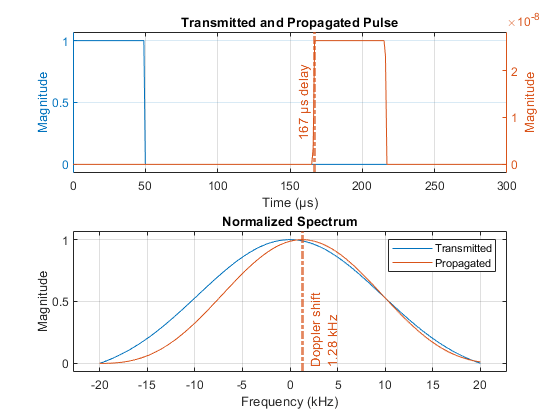
Visualize the transmitted and propagated pulses and their normalized spectra. The channel introduced a delay of 167 which corresponds to the 50 km range of the target divided by the speed of light.

[delay, dop] = helperPlotDelayAndDopplerShift(wav,y2ray,waveform.SampleRate);

estRange = delay*c*1e-3 % km

estRange =

   49.9954

The channel also applied a Doppler shift that corresponds to the range rate of the target. Compare the estimated value to the -200 m/s ground truth using the dop2speed and freq2wavelen functions.

estRangeRate = -dop2speed(dop,freq2wavelen(fc)) % m/s

estRangeRate =

 -201.9038

Multipath Fading

Calculate the signal loss suffered in this channel.

L_2ray = pow2db(bandpower(wav))-pow2db(bandpower(y2ray))

L_2ray =

  151.5888

Calculate the free-space path loss.

L_ref = fspl(norm(pos_target-pos_radar),c/fc)

L_ref =

  132.0069

The result suggests that in this configuration, the channel introduces an extra 19.6 dB loss to the received signal compared to the free space case. Now assume the target flies a bit higher at 1.8 km above the ground. Repeating the simulation above suggests that this time the ground reflection actually provides a 6 dB gain. Although free space path loss is essentially the same in the two scenarios, a 150 m move caused a 25.6 dB fluctuation in signal power.

pos_target = [50e3;0;1.8e3];
y2ray  = channel(wav,pos_radar,pos_target,vel_radar,vel_target);
L_2ray = pow2db(bandpower(wav))-pow2db(bandpower(y2ray))
L_ref  = fspl(norm(pos_target-pos_radar),c/fc)

L_2ray =

  126.0374


L_ref =

  132.0078

Increasing the bandwidth of a system increases the capacity of its channel. This enables higher data rates in communication systems and finer range resolutions for radar systems. The increased bandwidth can also improve robustness to multipath fading for both systems.

Typically, wideband systems operate with a bandwidth of greater than 5% of their center frequency. In contrast, narrowband systems operate with a bandwidth of 1% or less of the center frequency.

The narrowband channel in the preceding section was shown to be very sensitive to multipath fading. Slight changes in the target's height resulted in considerable signal losses.

Plot the fading loss for the channel by varying the height of the target across a span of operational heights for this radar system. Choose a span of heights from 1 km to 3 km.

% Simulate the signal fading at the target for heights from 1 km to 3 km
hTarget = linspace(1e3,3e3);
pos_target = repmat([50e3;0;1.6e3],[1 numel(hTarget)]);
pos_target(3,:) = hTarget;
vel_target = repmat(vel_target,[1 numel(hTarget)]);

release(channel);
y2ray = channel(repmat(wav,[1 numel(hTarget)]),pos_radar,pos_target,vel_radar,vel_target);

Plot the signal loss observed at the target.

L2ray = pow2db(bandpower(wav))-pow2db(bandpower(y2ray));

clf;
plot(hTarget,L2ray);
xlabel('Target Height (m)');
ylabel('One-Way Propagation Loss (dB)');
title('Multipath Fading Observed at the Target');
grid on;

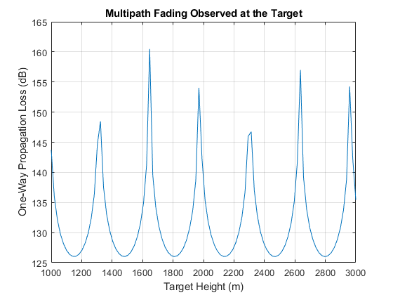
The sensitivity of the channel loss to target height for this narrowband system is clear. Deep signal fades occur at heights that are likely to be within the surveillance area of the radar.

Increasing the bandwidth of the channel can improve robustness to these multipath fades. To do this, use a wideband waveform with a bandwidth of 8% of the center frequency of the link.

bw = 0.08*fc;
pulse_width = 1/bw;
fs = 2*bw;

waveform = phased.RectangularWaveform('SampleRate',fs,'PRF',2000,'PulseWidth',pulse_width);
wav = waveform();

Use a wideband version of this channel model, widebandTwoRayChannel, to simulate multipath reflections of this wideband signal off of the ground between the radar and the target, and to compute the corresponding channel loss.

channel = widebandTwoRayChannel('PropagationSpeed',c,'OperatingFrequency',fc,'SampleRate',fs);

Simulate the signal at the target for various operational heights.

y2ray_wb = channel(repmat(wav,[1 numel(hTarget)]),pos_radar,pos_target,vel_radar,vel_target);
L2ray_wb = pow2db(bandpower(wav))-pow2db(bandpower(y2ray_wb));

hold on;
plot(hTarget,L2ray_wb);
hold off;
legend('Narrowband','Wideband');

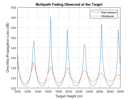
As expected, the wideband channel provides much better performance across a wide range of heights for the target. In fact, as the height of the target increases, the impact of multipath fading almost completely disappears. This is because the difference in propagation delay between the direct and bounce path signals is increasing, reducing the amount of coherence between the two signals when received at the target.

Conclusion

This example provides an overview of RF propagation losses due to atmospheric and weather effects. It also introduces multipath signal fluctuations due to ground bounces. It highlights functions and objects to simulate attenuation losses for narrowband and wideband single-bounce channels.

References

[1] Seybold, John S. Introduction to RF Propagation:
Seybold/Introduction to RF Propagation. Hoboken, NJ, USA: John Wiley &
Sons, Inc., 2005. https://doi.org/10.1002/0471743690

[2] Recommendation ITU-R P.838-3, 2005

[3] Recommendation ITU-R P.840-3, 2013

[4] Recommendation ITU-R P.676-10, 2013

[5] Recommendation ITU-R P.525-2, 1994

[6] Rain, A Water Resource (Pamphlet), U.S. Geological Survey, 1988

Supporting Functions

helperPlotPropagationFactor

function helperPlotPropagationFactor(R,F,Rd)

% Plot interference and diffraction region patches
[minF, maxF] = bounds(F(:));
maxF = ceil((maxF+10)/10)*10;
minF = floor((minF-10)/10)*10;
yPatch = [minF minF maxF maxF];
c1 = [0.3010 0.7450 0.9330];
c2 = [0 0.4470 0.7410];
clf % clear current figure
fill([R(1) Rd Rd R(1)]/1e3,yPatch,c1,'EdgeColor','none','FaceAlpha',0.25)
hold on
fill([Rd R(end) R(end) Rd]/1e3,yPatch,c2,'EdgeColor','none','FaceAlpha',0.25)

% Plot one-way propagation factor
set(gca,'ColorOrderIndex',1); % reset color index
plot(R/1e3,F);
ylim([minF maxF])
grid on;
xlabel('Range (km)');
ylabel('Propagation Factor (dB)');
title('One-Way Propagation Factor at 1 km above Surface');
legend('Interference Region', 'Diffraction Region',...
    'L-Band (1.06 GHz)', 'C-Band (5.7 GHZ)',...
    'Location','SouthWest')
hold off
end

helperPlotBlakeChart

function helperPlotBlakeChart(vcp,vcpang,N)
% Calculate refraction exponent
DelN = -7.32*exp(0.005577*N);
rexp = log(N./(N + DelN));

subplot(211)
blakechart(vcp{1},vcpang{1},'SurfaceRefractivity',N,'RefractionExponent',rexp);
legend('L-Band (1.06 GHz)')
xlabel('')
title ('Blake Chart - Antenna Height: 12 m')
subplot(212)
blakechart(vcp{2},vcpang{2},'SurfaceRefractivity',N,'RefractionExponent',rexp);
allc = get(gca,'Children');
set(allc(11),'Color',[0.8500 0.3250 0.0980]) % Change line color
title('')
legend('C-Band (5.7 GHz)')
end

helperPlotDelayAndDopplerShift

function [delay, dop] = helperPlotDelayAndDopplerShift(wav,y2ray,Fs)
% Plot transmitted and propagated pulse
t = 1e6*(0:numel(wav)-1)'/Fs;
subplot(211)
yyaxis left
plot(t,abs(wav))
ylabel('Magnitude')
yyaxis right
plot(t,abs(y2ray))
grid on
axis padded
xlim([0 300])
xlabel(['Time (' char(0x00B5) 's)'])
ylabel('Magnitude')
title('Transmitted and Propagated Pulse')

% Annotation
delay = midcross(abs(y2ray),t/1e6,'MidPercentReferenceLevel',80); % seconds
delay = delay(1);
xl = xline(1e6*delay,'-.',... % Annotation
    {[num2str(round(1e6*delay)),' ',char(0x00B5) 's delay']},'Color',[0.8500 0.3250 0.0980]);
xl.LabelVerticalAlignment = 'middle';
xl.LabelHorizontalAlignment = 'left';
xl.LineWidth = 2;

% Plot power spectrum
subplot(212)
[p,f] = pspectrum([wav y2ray],Fs,'FrequencyLimits',[-20e3 20e3]);
p = abs(p);
plot(1e-3*f,rescale(p,'InputMin',min(p),'InputMax',max(p)));
axis padded
grid on
[~,idx]=max(p);
dop = f(idx(2))-f(idx(1));   % Hz
xlabel('Frequency (kHz)')
ylabel('Magnitude')
title('Normalized Spectrum')

xl = xline(1e-3*dop,'-.',... % Annotation
    {'Doppler shift',[num2str(round(dop)*1e-3) ' kHz']},'Color',[0.8500 0.3250 0.0980]);
xl.LabelVerticalAlignment = 'bottom';
xl.LineWidth = 2;
legend('Transmitted','Propagated')
end

helperCombineEnvLosses

function [PLdB, PLdBNorm] = helperCombineEnvLosses(R,freq,anht,tgtht,htsd,beta0,elbw)
% Calculate the combined environment losses
numHt = numel(tgtht);
numR = numel(R);
F = zeros(numHt,numR);
for ih = 1:numHt
    F(ih,:) = radarpropfactor(R, freq, anht, tgtht(ih),...
    'SurfaceHeightStandardDeviation',htsd,'SurfaceSlope',beta0,...
    'ElevationBeamwidth', elbw);
end

% Free space spreading loss
Lspl_dB = 2*fspl(R,freq2wavelen(freq));  % Factor of 2 for two-way

% Perform tropospheric losses calculation for a subset of elevation angles,
% since the ray refracting can take a long time.
numEl = 10;
minEl = height2el(tgtht(1),anht,R(end)); % Min elevation angle (deg)
maxEl = height2el(tgtht(end),anht,R(1)); % Max elevation angle (deg)
elSubset = linspace(minEl,maxEl,numEl);
LtropoSubset = zeros(numEl,numR);
for ie = 1:numEl
    LtropoSubset(ie,:) = tropopl(R,freq,anht,elSubset(ie));
end
% Interpolate tropospheric losses for all elevation angles of interest
Ltropo = zeros(numHt,numR);
for ir = 1:numR
    el = height2el(tgtht,anht,R(ir));
    Ltropo(:,ir) = interp1(elSubset,LtropoSubset(:,ir),el);
end

PLdB = 2*F - Lspl_dB - Ltropo;           % Factor of 2 for two-way
PLdBNorm = PLdB - max(PLdB(:));
end

helperPlotCombinedEnvLosses

function helperPlotCombinedEnvLosses(Rkm,freq,anht,tgtht,PLdBNorm)
% Plot combined losses for different heights and ranges
hP = pcolor(Rkm,tgtht,PLdBNorm);
set(hP, 'EdgeColor', 'none');
title([num2str(freq/1e9) ' GHz S-Band Radar'])
subtitle([num2str(round(anht)) ' m above water'])
xlabel('Range (km)')
ylabel('Height (m)')
colormap('jet');
clim([-150 0])
hC = colorbar;
hC.Label.String = 'Normalized Two-Way Propagation Loss (dB)';
end