Radar Surveillance Scan Pattern Tutorial

R2026b

Since R2026b

This example shows how to use radarScanController to simulate sector and raster surveillance scan patterns. Surveillance radars use scan patterns to systematically search a region of interest for targets. The choice of scan pattern — sector vs. raster — and scan mode — mechanical vs. electronic — depends on the antenna beam shape, the required coverage volume, and the desired revisit rate. This example demonstrates these configurations using a bistatic radar scenario that visualizes beam positions and the corresponding variation in received signal power as the transmit beam sweeps past the bistatic receiver.

Create a Bistatic Radar Scenario

Create a bistatic transmitter with a fan beam having a 10-degree azimuth beamwidth and a 30-degree elevation beamwidth.

freq = 300e6;
txAnt = phased.SincAntennaElement(Beamwidth=[10 30]);
txRdr = bistaticTransmitter(TransmitAntenna=phased.Radiator(Sensor=txAnt,OperatingFrequency=freq));

Create a bistatic receiver using an isotropic antenna element. This simplifies the received signal power plots that follow, since only the transmit antenna pattern contributes to the variation in received power as the beam scans past the receiver.

rxAnt = phased.IsotropicAntennaElement;
rxRdr = bistaticReceiver(ReceiveAntenna=phased.Collector(Sensor=rxAnt,OperatingFrequency=freq));

Use the local helperCreateScenario function to create a simple bistatic radar scenario. The variation in the transmitter's direct-path signal illustrates how the transmit and receive beam patterns combine as the transmit beam sweeps across the receive array.

[scnro,txPlat,rxPlat,tp,plotScnro] = helperCreateScenario();

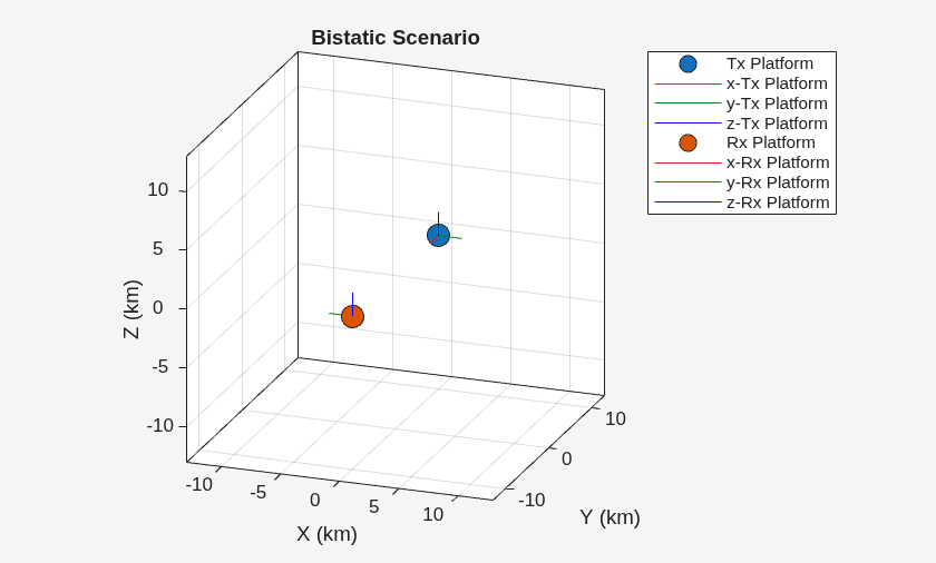
Figure Bistatic Scenario contains an axes object. The axes object with title Bistatic Scenario, xlabel X (km), ylabel Y (km) contains 8 objects of type line. One or more of the lines displays its values using only markers These objects represent Tx Platform, x-Tx Platform, y-Tx Platform, z-Tx Platform, Rx Platform, x-Rx Platform, y-Rx Platform, z-Rx Platform.

Mechanically Scan a 1D Surveillance Sector

A surveillance sector scan sweeps out a 1D angular sector. Create a mechanical sector scan controller that scans the azimuth sector from -30 to 30 degrees. Set the scan duration to 31 pulse repetition intervals (PRIs) so the beam sweeps slowly enough to capture the full transmit antenna pattern — including the mainbeam and sidelobes — as it traverses the receive antenna's location.

pri = 1/txRdr.Waveform.PRF;
txScnr = radarScanController("Mechanical","Sector",AzimuthLimits=[-30 30],ScanDuration=31*pri)

txScnr = 
  MechanicalSectorScanner with properties:

     AzimuthLimits: [-30 30]
      ScanDuration: 0.0031
         ScanReset: "Return"
    ReturnDuration: 0
    ScanRateSource: "Auto"
         ScanAngle: -30
          ScanTime: 0

Use coverageConfig and coveragePlotter to plot the initial scan position in the scenario plot.

txCovCfg = coverageConfig(txScnr)

txCovCfg = struct with fields:
          Index: 1
      LookAngle: [-30 0]
    FieldOfView: [0 0]
     ScanLimits: [-30 30]
          Range: 1
       Position: [0 0 0]
    Orientation: [1×1 quaternion]

Update the returned coverage configuration to include information about the transmit radar and platform associated with this scanner.

txCovCfg.Index = txPlat.PlatformID;
txCovCfg.Range = 20e3;
txCovCfg.FieldOfView = txRdr.TransmitAntenna.Sensor.Beamwidth;
txCovCfg.Position = txPlat.Position;
txCovCfg.Orientation = quaternion(txPlat.Orientation,"eulerd","ZYX","frame");

txCovPltr = coveragePlotter(tp,DisplayName="Tx Coverage");
plotCoverage(txCovPltr,txCovCfg);

The receive platform does not scan its antenna. Create a stationary scanner by setting both azimuth limits to the same value — this forces the scanner to stare at a fixed angle (0 degrees in this case). A stationary scanner still integrates with coverageConfig and the simulation loop, simplifying the coverage plotting code.

rxScnr = radarScanController("Mechanical","Sector",AzimuthLimits=[0 0])

rxScnr = 
  MechanicalSectorScanner with properties:

    AzimuthLimits: [0 0]
        ScanAngle: 0
         ScanTime: 0

Add the receive antenna's coverage to the scenario visualization.

rxCovCfg = coverageConfig(rxScnr);
rxCovCfg.Index = rxPlat.PlatformID;
rxCovCfg.Range = 3e3;
rxCovCfg.FieldOfView = [360 180]; % Isotropic antenna coverage
rxCovCfg.Position = rxPlat.Position;
rxCovCfg.Orientation = quaternion(rxPlat.Orientation,"eulerd","ZYX","frame");

rxCovPltr = coveragePlotter(tp,DisplayName="Rx Coverage");
plotCoverage(rxCovPltr,rxCovCfg);

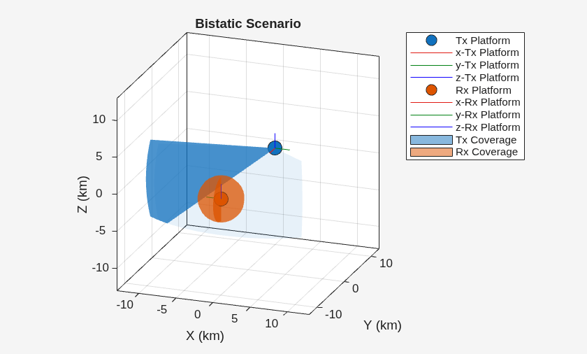
Figure Bistatic Scenario contains an axes object. The axes object with title Bistatic Scenario, xlabel X (km), ylabel Y (km) contains 10 objects of type line, patch. One or more of the lines displays its values using only markers These objects represent Tx Platform, x-Tx Platform, y-Tx Platform, z-Tx Platform, Rx Platform, x-Rx Platform, y-Rx Platform, z-Rx Platform, Tx Coverage, Rx Coverage.

The plot above shows the transmit antenna's field of view as the dark blue region and its scan limits as the lighter blue region. The transmit antenna uses a fan beam that scans out the 1D azimuth sector. The receive antenna uses an isotropic antenna element, so it does not need to scan — its field of view is represented as the red sphere centered on the receive platform. The ranges assigned to the transmit and receive coverage regions are purely for illustrative purposes.

Run two complete scans using the local runScenario function defined below. This function advances the scenario, updates the theater plot, and plots the received signal power over time. It also superimposes the expected sinc antenna pattern at each PRI's scan angle, showing how the scan mode and transmit antenna pattern modulate the received signal.

scnro.StopTime = scnro.SimulationTime + 2*txScnr.ScanDuration;

function runScenario(scnro,scnroName,txPlat,txRdr,txScnr,txCovPltr,txCovCfg,rxPlat,rxRdr,rxScnr,rxCovPltr,rxCovCfg,tp,plotScnro)

% Set scenario update rate to match transmitter's waveform
if scnro.SimulationStatus=="NotStarted"
    scnro.UpdateRate = txRdr.Waveform.PRF;
end

% Create signal plot for received signal
fov = txRdr.TransmitAntenna.Sensor.Beamwidth;
patOffset = -30; % Offset used to align sinc pattern with received signal power
patFcn = @(ang)helperSincPattern(ang,fov) + patOffset;

% Compute delay required to align sinc pattern truth with center of
% transmitted and propagated pulses to the receiver
pw = txRdr.Waveform.PulseWidth;
dly = range2time(norm(rxPlat.Position-txPlat.Position))/2; % divide-by-two to remove monostatic 2-way assumption applied in range2time

tl = tp.Parent.Parent;
title(tl,scnroName);

plotSignalPower = helperSignalPowerPlot(tl,dly+pw/2,patFcn);
plotTxCovHistory = helperCoverageHistoryPlot(txCovPltr);

isRunning = true;
while isRunning
    isRunning = advance(scnro);
    plotTxCovHistory(txCovCfg);

    % Update the scanners to the current simulation time
    txAng = scan(txScnr,scnro.SimulationTime);
    rxAng = scan(rxScnr,scnro.SimulationTime);

    % Update the coverage plots for the scanners
    txCovCfg = coverageConfig(txScnr,Index=txCovCfg.Index,FieldOfView=txCovCfg.FieldOfView,Range=txCovCfg.Range);
    txCovCfg.Orientation = quaternion(txPlat.Orientation,"eulerd","ZYX","frame");
    txCovCfg.Position = txPlat.Position;
    plotCoverage(txCovPltr,txCovCfg);

    rxCovCfg = coverageConfig(rxScnr,Index=rxCovCfg.Index,FieldOfView=rxCovCfg.FieldOfView,Range=rxCovCfg.Range);
    rxCovCfg.Orientation = quaternion(rxPlat.Orientation,"eulerd","ZYX","frame");
    rxCovCfg.Position = rxPlat.Position;
    plotCoverage(rxCovPltr,rxCovCfg);

    % Update scenario theater plot
    plotScnro();

    % Compute paths
    [txPose,rxPose,tgtPoses] = helperPlatformTruth(scnro,txPlat,rxPlat);
    propPaths = bistaticFreeSpacePath(txRdr.TransmitAntenna.OperatingFrequency,txPose,rxPose,tgtPoses, ...
        TransmitterMountingAngles=paddata(txAng,[1 3]).*[1 -1 1], ... % Convert scan angle(s) [az -el 0] to mounting angles [yaw pitch roll]
        ReceiverMountingAngles=paddata(rxAng,[1 3]).*[1 -1 1]);       % For sector scan, only az is returned, for raster scanners both [az el] is returned

    % Transmit
    [txSig,txInfo] = transmit(txRdr,propPaths,scnro.SimulationTime);

    % Receive collected transmissions
    [rxSig,rxInfo] = receive(rxRdr,txSig,txInfo,propPaths);

    % Plot the received signal power
    plotSignalPower(rxSig,rxInfo,txAng,isScanDone(txScnr));
end
end

runScenario(scnro,"Mechanical Azimuth Sector Scan",txPlat,txRdr,txScnr,txCovPltr,txCovCfg,rxPlat,rxRdr,rxScnr,rxCovPltr,rxCovCfg,tp,plotScnro);

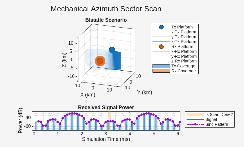
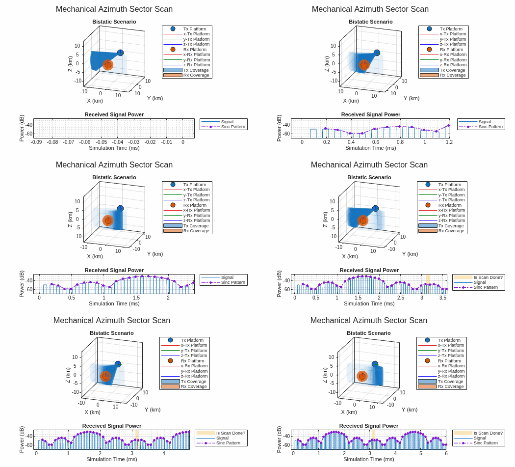
The top plot shows the transmit beam scanning out the 1D azimuth sector. The bottom plot shows the transmitted signal power received by the bistatic receiver. The gain of the sinc antenna element pattern in the direction of the bistatic receiver is superimposed over the received signal power to show how the two relate. When the scanner reaches the end of the sector, a light yellow region in the signal power plot indicates that the scan is done.

Return Scan Reset

By default, the mechanical sector scanner returns to its start position instantaneously. In practice, a mechanical scanner returns quickly but not instantaneously. Use the ReturnDuration property to model a return time that is one-quarter of the scan duration.

% Release the scanner so that the property can be updated
release(txScnr);
txScnr.ReturnDuration = txScnr.ScanDuration/4;

Restart the scenario and reset the radars by releasing their corresponding objects so the scenario can be run again.

restart(scnro);
resetRadars(txRdr,txScnr,rxRdr,rxScnr);

function resetRadars(varargin)
% Calls release on the radar objects to reset their state for simulation
for m = 1:nargin
    release(varargin{m});
end
end

Run the simulation again.

scnro.StopTime = 2*(txScnr.ScanDuration + txScnr.ReturnDuration);
runScenario(scnro,"Mechanical Sector Return Scan Reset",txPlat,txRdr,txScnr,txCovPltr,txCovCfg,rxPlat,rxRdr,rxScnr,rxCovPltr,rxCovCfg,tp,plotScnro);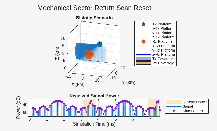

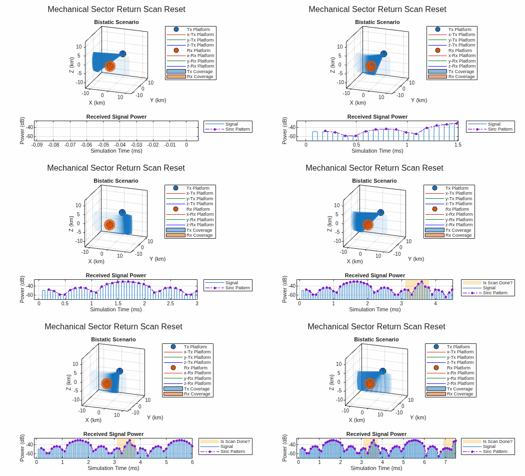
This plot shows a similar scan pattern as before, but the scan-done region (light yellow) is now wider, reflecting the return duration. For mechanical scanners, the scan is marked done for the entire return phase. As the scanner returns to its starting position, it quickly sweeps the mainbeam of its sinc pattern across the bistatic receiver, producing the abrupt peak in received signal power visible during the return.

Reverse Scan Reset

Mechanical scanners support two reset modes. The previous simulation used "Return" mode, which returns the scanner to its start position as quickly as possible. Because the scanner moves faster during the return, detections cannot reliably be made during this phase. A "Reverse" reset avoids this lost time by retracing the scan pattern in reverse at the same speed as the forward scan. Set ScanReset to "Reverse" and rerun the simulation.

release(txScnr);
txScnr.ScanReset ="Reverse";

restart(scnro);
resetRadars(txRdr,txScnr,rxRdr,rxScnr);
scnro.StopTime = 4*txScnr.ScanDuration;
runScenario(scnro,"Mechanical Sector Reverse Scan Reset",txPlat,txRdr,txScnr,txCovPltr,txCovCfg,rxPlat,rxRdr,rxScnr,rxCovPltr,rxCovCfg,tp,plotScnro);

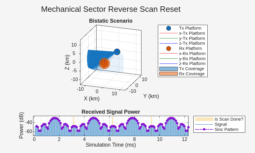
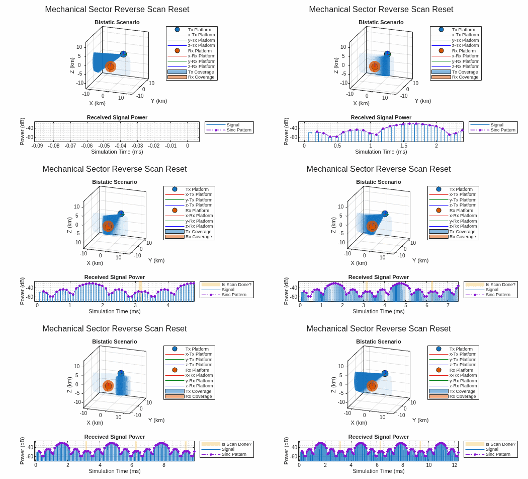
This plot shows the transmitter scanning the sector in reverse at the same speed upon reaching the end of its scan limits. In this reset mode, the scan is marked done only when the scanner reaches the end of the limits.

360-degree Scan

The azimuth limits can span up to 360 degrees. When the span equals exactly 360 degrees, the scanner wraps continuously — the final scan position coincides with the start, so no reset is needed. The scan limits define both the first scan angle and the scan direction. Set the scan limits to [-90 270] so the scan starts at -90 degrees azimuth and advances toward 270 degrees. Because these limits span 360 degrees, the scanner wraps continuously.

release(txScnr)
txScnr.AzimuthLimits = [-90 270];

Use the local newCoveragePlotter function to create a new coverage plotter for the new scan pattern limits on the transmitter.

txCovPltr = newCoveragePlotter(txCovPltr);

function pltr = newCoveragePlotter(pltr)
clearData(pltr)
tp = pltr.ParentPlot;
name = pltr.DisplayName;
tag = pltr.Tag;
delete(pltr)
pltr = coveragePlotter(tp,DisplayName=name,Tag=tag);
end

Set the scan duration to 91 PRIs to illustrate the transmit antenna pattern across the much larger scan angle.

txScnr.ScanDuration = 91*pri;

The displayed object no longer shows ScanReset or ReturnDuration since these properties do not apply to a 360-degree scan.

disp(txScnr)

  MechanicalSectorScanner with properties:

     AzimuthLimits: [-90 270]
      ScanDuration: 0.0091
    ScanRateSource: "Auto"
         ScanAngle: -90
          ScanTime: 0.0124

Run the simulation to demonstrate the 360-degree scan mode.

restart(scnro);
resetRadars(txRdr,txScnr,rxRdr,rxScnr);
scnro.StopTime = 2*txScnr.ScanDuration;
runScenario(scnro,"Mechanical 360-degree Sector Scan",txPlat,txRdr,txScnr,txCovPltr,txCovCfg,rxPlat,rxRdr,rxScnr,rxCovPltr,rxCovCfg,tp,plotScnro);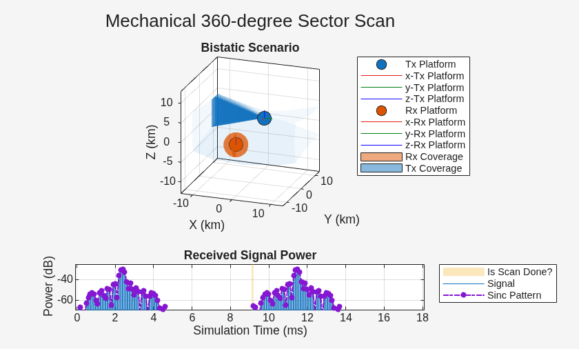

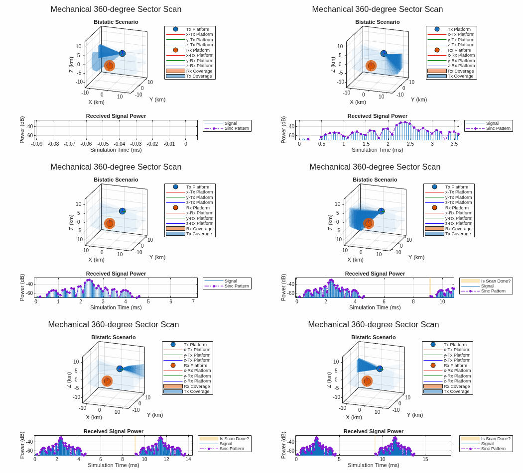
This plot shows two complete scans of the 360-degree sector. The scan starts at -90 degrees and advances in the direction of increasing azimuth angle, consistent with the scan limits.

Scan Direction

The order of the scan limits controls both the initial scan angle and the scan direction. The previous scan started at -90 degrees and scanned toward 270 degrees. Reverse the scan direction while keeping the same initial angle.

release(txScnr)
txScnr.AzimuthLimits = -90 + [0 -360];

Run the simulation to demonstrate the reversed scan direction.

restart(scnro);
resetRadars(txRdr,txScnr,rxRdr,rxScnr);
runScenario(scnro,"Mechanical Sector Reverse Scan Direction",txPlat,txRdr,txScnr,txCovPltr,txCovCfg,rxPlat,rxRdr,rxScnr,rxCovPltr,rxCovCfg,tp,plotScnro);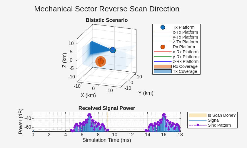

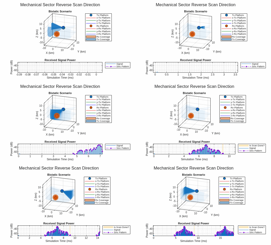
The scan pattern starts at the same angle as the previous 360-degree scan, but now sweeps in the direction of decreasing azimuth angle. This illustrates how the scan limits control both the initial scan angle and the scan direction.

Stationary Scanner

A scanner can stare at a fixed angle by setting both of its scan limits to the same value. This produces a stationary scanner that never advances its beam position. Stationary scanners are useful for modeling fixed-beam radars or for holding one end of a bistatic link at a constant look angle while the other end scans.

release(txScnr)
txScnr.AzimuthLimits = [15 15];

The displayed object shows only AzimuthLimits, ScanAngle, and ScanTime — scan timing and reset properties are hidden because they have no effect when the scanner does not move.

restart(scnro);
resetRadars(txRdr,txScnr,rxRdr,rxScnr);
txCovPltr = newCoveragePlotter(txCovPltr);
txCovCfg = coverageConfig(txScnr);
txCovCfg.Index = txPlat.PlatformID;
txCovCfg.Range = 20e3;
txCovCfg.FieldOfView = txRdr.TransmitAntenna.Sensor.Beamwidth;
txCovCfg.Position = txPlat.Position;
txCovCfg.Orientation = quaternion(txPlat.Orientation,"eulerd","ZYX","frame");

scnro.StopTime = 10*pri;
runScenario(scnro,"Mechanical Stationary Scanner",txPlat,txRdr,txScnr,txCovPltr,txCovCfg,rxPlat,rxRdr,rxScnr,rxCovPltr,rxCovCfg,tp,plotScnro);

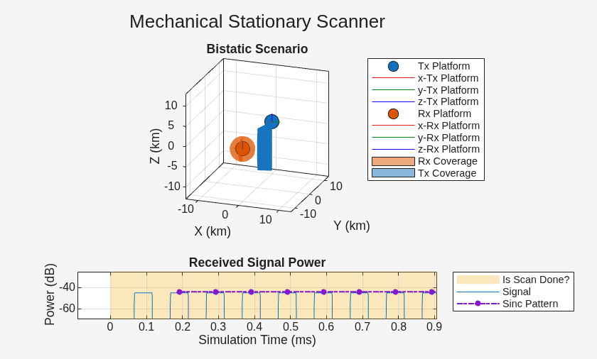
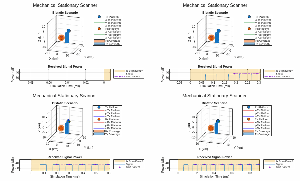
The beam remains fixed at 15 degrees azimuth for the entire simulation. Since the receiver is located at 0 degrees azimuth — outside the mainbeam — the received signal power reflects only the sidelobe level of the transmit antenna pattern. Also, because the scan position never changes, the scan is always marked as done.

Mechanically Scan a 2D Surveillance Volume

A sector scan works well when the beam is fan-shaped — narrow in azimuth but wide in elevation — since the wide elevation beamwidth captures targets across a range of altitudes. When the radar uses a pencil beam that is narrow in both dimensions, a different scan pattern is needed. Common 2D surveillance scan patterns include spiral, helical, nodding, and Palmer scans. In addition to these, a basic but widely used pattern known as a raster scan can cover the full surveillance volume. Create a mechanical raster scan controller that scans from -30 to 30 degrees in azimuth and -5 to 25 degrees in elevation.

txScnr = radarScanController("Mechanical","Raster",AzimuthLimits=[-30 30],ElevationLimits=[-5 25])

txScnr = 
  MechanicalRasterScanner with properties:

      AzimuthLimits: [-30 30]
    ElevationLimits: [-5 25]
       ScanDuration: 1
            NumBars: 2
          Alignment: "Azimuth"
          ScanReset: "Return"
     ReturnDuration: 0
     ScanRateSource: "Auto"
          ScanAngle: [-30 -5]
           ScanTime: 0

The raster scanner sweeps along its primary scan direction, defined by the Alignment property. When it reaches the end of the primary axis (azimuth in this case), it steps along the secondary axis to the next raster bar. Raster bars are spaced evenly between the secondary limits, and the scanner reverses its primary scan direction each time it steps to a new bar.

Define a pencil beam with a 10-degree beamwidth in both azimuth and elevation. The 30-degree elevation span requires 30/10 + 1 = 4 raster bars to cover the full surveillance volume.

fov = [10 10]; % [az el] degrees
release(txRdr)
txRdr.TransmitAntenna.Sensor.Beamwidth = fov;

txScnr.NumBars = floor(diff(txScnr.ElevationLimits)/fov(2)) + 1

txScnr = 
  MechanicalRasterScanner with properties:

      AzimuthLimits: [-30 30]
    ElevationLimits: [-5 25]
       ScanDuration: 1
            NumBars: 4
          Alignment: "Azimuth"
          ScanReset: "Return"
     ReturnDuration: 0
     ScanRateSource: "Auto"
          ScanAngle: [-30 -5]
           ScanTime: 0

Set the scan duration so that 31 PRIs are transmitted for each raster bar.

txScnr.ScanDuration = 31 * pri * txScnr.NumBars;

Use coverageConfig and coveragePlotter to plot the initial scan position in the scenario plot.

txCovPltr = newCoveragePlotter(txCovPltr);
txCovCfg = coverageConfig(txScnr)

txCovCfg = struct with fields:
          Index: 1
      LookAngle: [-30 -5]
    FieldOfView: [0 0]
     ScanLimits: [2×2 double]
          Range: 1
       Position: [0 0 0]
    Orientation: [1×1 quaternion]

Update the returned coverage configuration to include information about the transmit radar and platform associated with this scanner.

txCovCfg.Index = txPlat.PlatformID;
txCovCfg.Range = 20e3;
txCovCfg.FieldOfView = fov;
txCovCfg.Position = txPlat.Position;
txCovCfg.Orientation = quaternion(txPlat.Orientation,"eulerd","ZYX","frame");

Run one complete raster scan.

restart(scnro);
resetRadars(txRdr,txScnr,rxRdr,rxScnr);

scnro.StopTime = txScnr.ScanDuration + 2 * pri; % scan past the end to see the end of scan marker
runScenario(scnro,"Mechanical Azimuth Raster Scan",txPlat,txRdr,txScnr,txCovPltr,txCovCfg,rxPlat,rxRdr,rxScnr,rxCovPltr,rxCovCfg,tp,plotScnro);

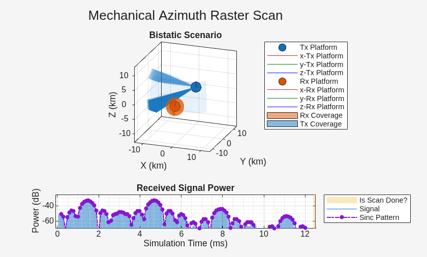
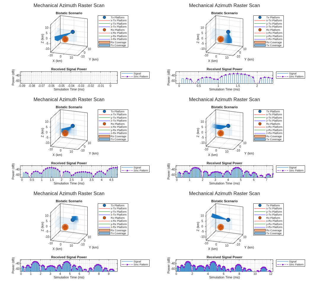
This plot shows the mechanical azimuth raster scan pattern as it scans across 4 raster bars. The received signal power peaks decrease as the raster bars move away from the receiver in elevation.

Raster Alignment

Choose the primary scan direction based on whichever axis has the larger span — this minimizes the number of raster bars. When the elevation span exceeds the azimuth span, set Alignment to "Elevation". Configure the scanner to scan -10 to 10 degrees in azimuth and -5 to 30 degrees in elevation.

release(txScnr)
txScnr.AzimuthLimits = [-10 10];
txScnr.ElevationLimits = [-5 30];
txScnr.Alignment = "Elevation";
txCovPltr = newCoveragePlotter(txCovPltr);

Compute the number of raster bars from the azimuth span and beamwidth.

txScnr.NumBars = floor(diff(txScnr.AzimuthLimits)/fov(1)) + 1

txScnr = 
  MechanicalRasterScanner with properties:

      AzimuthLimits: [-10 10]
    ElevationLimits: [-5 30]
       ScanDuration: 0.0124
            NumBars: 3
          Alignment: "Elevation"
          ScanReset: "Return"
     ReturnDuration: 0
     ScanRateSource: "Auto"
          ScanAngle: [-10 -5]
           ScanTime: 0.0126

Run the simulation with elevation alignment.

restart(scnro);
resetRadars(txRdr,txScnr,rxRdr,rxScnr);

scnro.StopTime = txScnr.ScanDuration + 2 * pri; % scan past the end to see the end of scan marker
runScenario(scnro,"Mechanical Elevation Raster Scan",txPlat,txRdr,txScnr,txCovPltr,txCovCfg,rxPlat,rxRdr,rxScnr,rxCovPltr,rxCovCfg,tp,plotScnro);

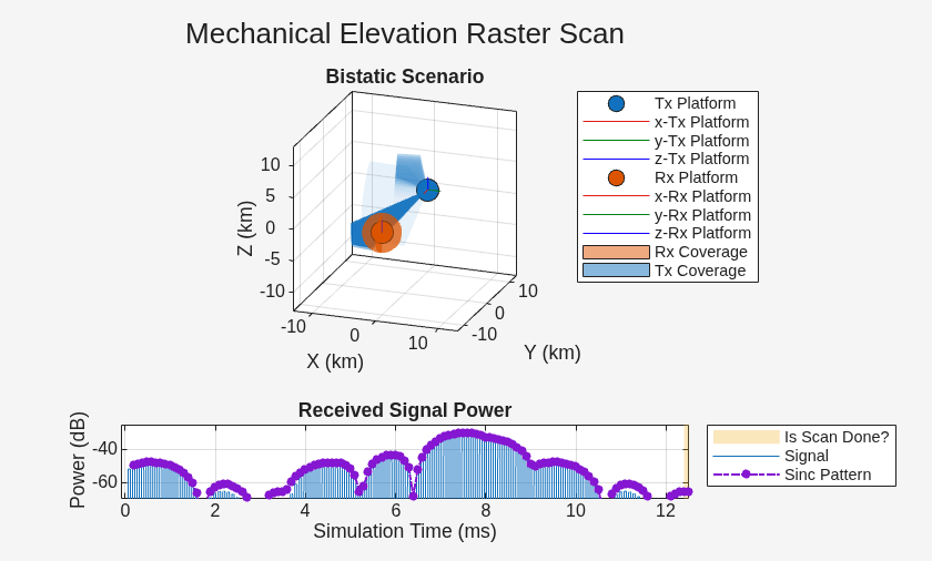
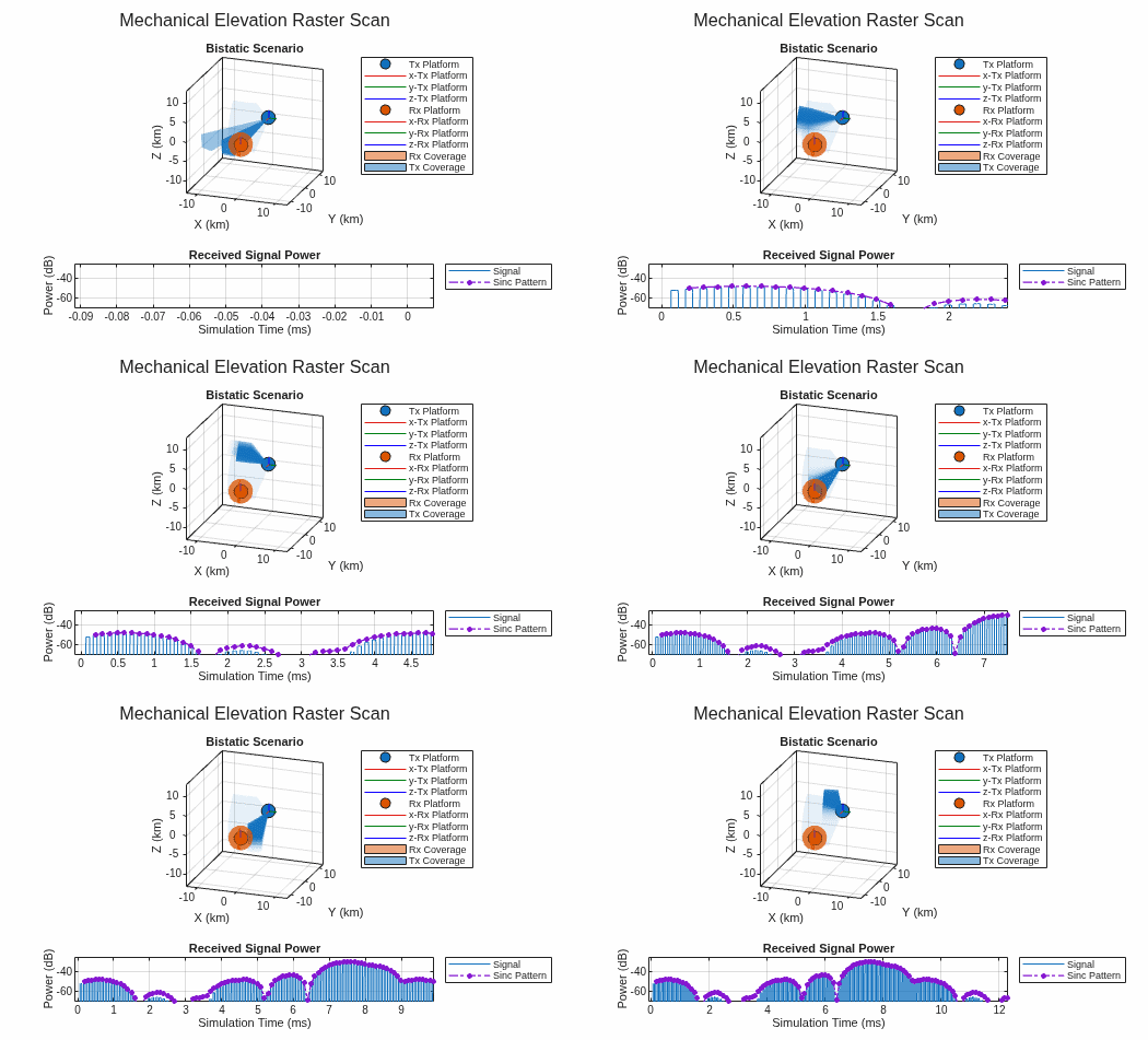
This plot shows a mechanical elevation raster scan pattern. The transmitter's sinc antenna element pattern now sweeps in elevation across the receiver. The peak in the received signal power corresponds to the raster bar at the receiver's azimuth.

360-degree Raster Scan

The ScanReset, ReturnDuration, and scan direction behaviors work the same way as for the sector scanner and are not repeated here. However, the 360-degree raster pattern introduces multi-bar wrapping that is worth illustrating. Configure the scanner to scan a full 360-degree azimuth sector between -5 and 15 degrees elevation.

release(txScnr)
txScnr.AzimuthLimits = [0 360];
txScnr.ElevationLimits = [-5 15];
txScnr.Alignment = "Azimuth";
txCovPltr = newCoveragePlotter(txCovPltr);

Compute the number of raster bars from the elevation span and beamwidth.

txScnr.NumBars = floor(diff(txScnr.ElevationLimits)/fov(2)) + 1;
txScnr.ScanDuration = 91 * pri * txScnr.NumBars

txScnr = 
  MechanicalRasterScanner with properties:

      AzimuthLimits: [0 360]
    ElevationLimits: [-5 15]
       ScanDuration: 0.0273
            NumBars: 3
          Alignment: "Azimuth"
          ScanReset: "Return"
     ReturnDuration: 0
     ScanRateSource: "Auto"
          ScanAngle: [0 -5]
           ScanTime: 0.0126

Run the 360-degree raster scan.

restart(scnro);
resetRadars(txRdr,txScnr,rxRdr,rxScnr);

scnro.StopTime = txScnr.ScanDuration + 2 * pri; % scan past the end to see the end of scan marker
runScenario(scnro,"Mechanical 360-degree Raster Scan",txPlat,txRdr,txScnr,txCovPltr,txCovCfg,rxPlat,rxRdr,rxScnr,rxCovPltr,rxCovCfg,tp,plotScnro);

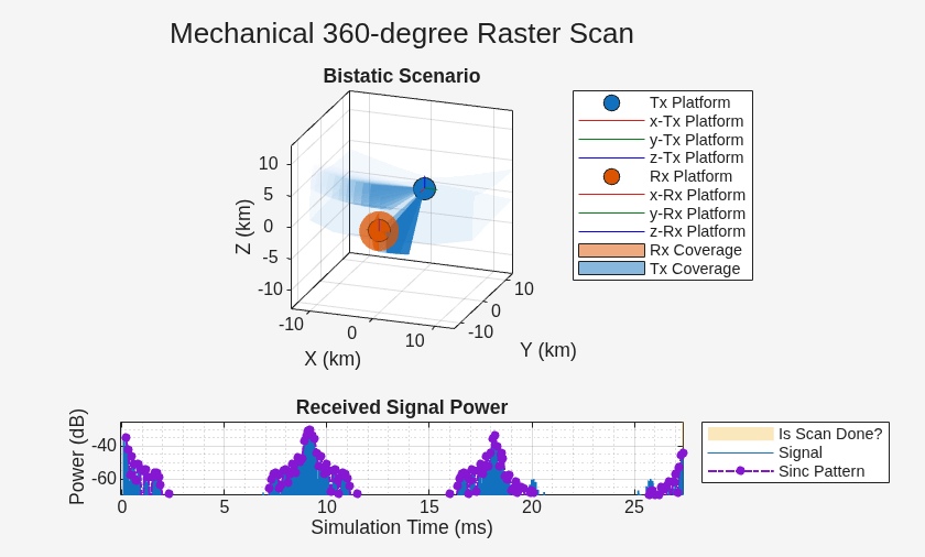
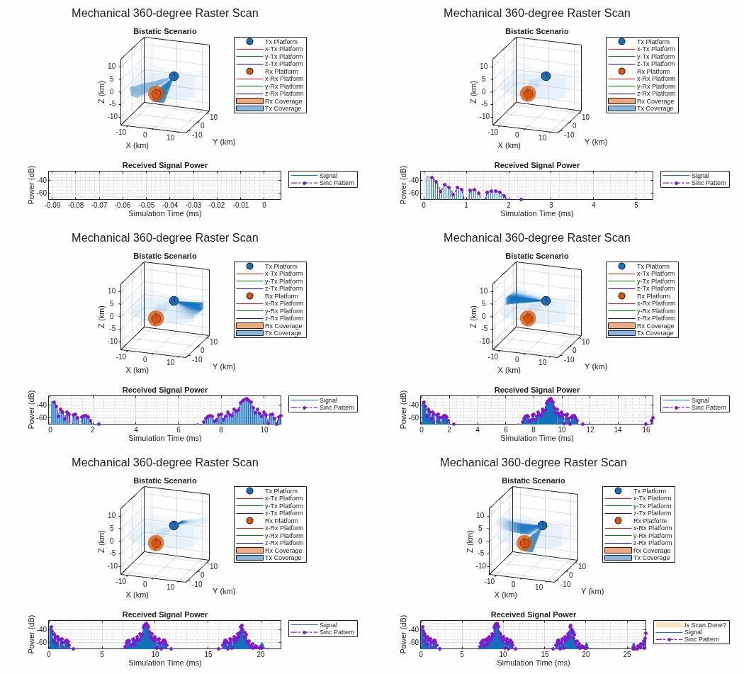
This plot shows the 360-degree mechanical raster scan using 3 raster bars. The transition between raster bars occurs at 0 degrees azimuth, which coincides with the azimuth of the receiver.

Electronically Scan a 1D Surveillance Sector

Electronic scanners steer the beam using a phased array rather than physically rotating an antenna. Unlike mechanical scanners, which sweep continuously, electronic scanners jump instantaneously between discrete angular positions and dwell at each position for a fixed time before advancing to the next. The StepAngle property defines the angular spacing between positions. Because the beam repositions instantaneously, electronic scanners have no return duration or reversal penalty — the beam simply jumps to its next position regardless of distance.

Create an electronic sector scanner that covers the same 60-degree azimuth sector used previously. Set StepAngle to 5 degrees, producing 13 discrete scan positions.

release(txRdr)
txRdr.TransmitAntenna.Sensor.Beamwidth = [10 30];
fov = txRdr.TransmitAntenna.Sensor.Beamwidth;

txScnr = radarScanController("Electronic","Sector",AzimuthLimits=[-30 30],StepAngle=5)

txScnr = 
  ElectronicSectorScanner with properties:

      AzimuthLimits: [-30 30]
       ScanDuration: 1
          StepAngle: 5
    DwellTimeSource: "Auto"
          ScanAngle: -30
           ScanTime: 0

The scanner computes the dwell time at each position by dividing ScanDuration by the number of positions. Set the scan duration to 26 PRIs so each of the 13 positions dwells for 2 PRIs.

txScnr.ScanDuration = 26*pri;

Set up the coverage plot and run two complete scans of the azimuth sector.

txCovPltr = newCoveragePlotter(txCovPltr);
txCovCfg = coverageConfig(txScnr);
txCovCfg.Index = txPlat.PlatformID;
txCovCfg.Range = 20e3;
txCovCfg.FieldOfView = fov;
txCovCfg.Position = txPlat.Position;
txCovCfg.Orientation = quaternion(txPlat.Orientation,"eulerd","ZYX","frame");

restart(scnro);
resetRadars(txRdr,txScnr,rxRdr,rxScnr);
scnro.StopTime = 2*txScnr.ScanDuration;
runScenario(scnro,"Electronic Sector Scan",txPlat,txRdr,txScnr,txCovPltr,txCovCfg,rxPlat,rxRdr,rxScnr,rxCovPltr,rxCovCfg,tp,plotScnro);

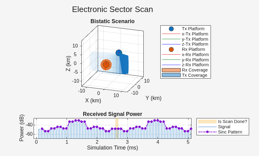
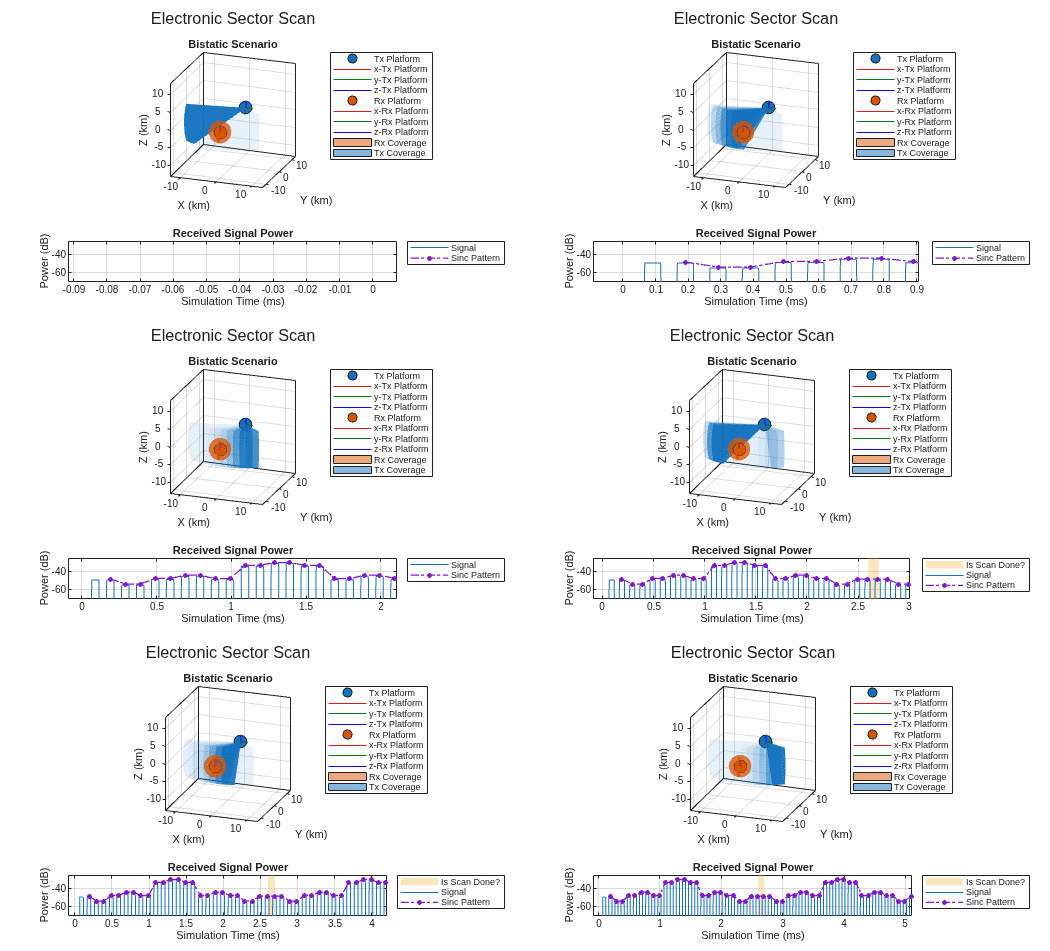
The received signal power plot shows a staircase pattern rather than a smooth sweep. Each flat segment corresponds to the beam dwelling at a fixed position for 2 PRIs before jumping to the next. Unlike mechanical scanners, which change position continuously, electronic scanners change position discretely — jumping instantaneously as the simulation time advances.

Dwell Time Configuration

By default, DwellTimeSource is "Auto" and the scanner computes the dwell time from ScanDuration and the number of positions. Set DwellTimeSource to "Property" to specify DwellTime directly — the scan duration then equals the dwell time multiplied by the number of positions. Set the dwell time to 4 PRIs per position.

release(txScnr);
txScnr.DwellTimeSource = "Property";
txScnr.DwellTime = 4*pri;
disp(txScnr)

  ElectronicSectorScanner with properties:

      AzimuthLimits: [-30 30]
          StepAngle: 5
    DwellTimeSource: "Property"
          DwellTime: 4.0000e-04
          ScanAngle: -30
           ScanTime: 0.0052

With DwellTimeSource set to "Property", ScanDuration no longer appears in the display since the dwell time and number of positions implicitly define it.

restart(scnro);
resetRadars(txRdr,txScnr,rxRdr,rxScnr);
scnro.StopTime = 2*txScnr.ScanDuration;
runScenario(scnro,"Electronic Dwell Time",txPlat,txRdr,txScnr,txCovPltr,txCovCfg,rxPlat,rxRdr,rxScnr,rxCovPltr,rxCovCfg,tp,plotScnro);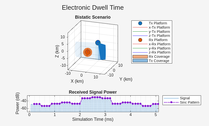

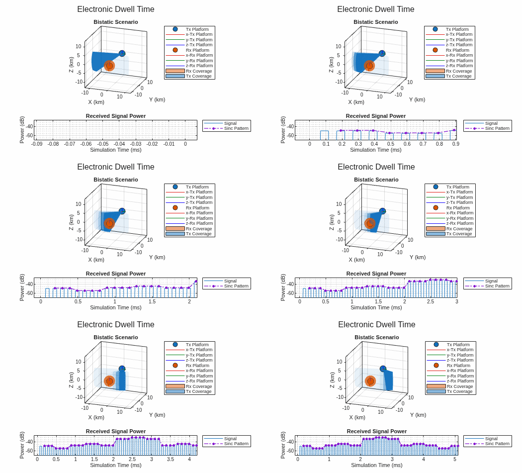
The longer dwell time produces wider staircase steps in the signal power plot, with 4 PRIs of constant power at each position.

Electronically Scan a 2D Surveillance Volume

Electronic raster scanners extend the sector pattern into a 2D surveillance volume by stacking scan bars along a secondary axis, just as their mechanical counterparts do. The NumBars and Alignment properties work the same way. Create an electronic raster scanner with a pencil beam to scan a surveillance volume.

release(txRdr)
txRdr.TransmitAntenna.Sensor.Beamwidth = [10 10];
fov = [10 10];

txScnr = radarScanController("Electronic","Raster", ...
    AzimuthLimits=[-30 30], ...
    ElevationLimits=[-5 25], ...
    StepAngle=10, ...
    NumBars=4)

txScnr = 
  ElectronicRasterScanner with properties:

      AzimuthLimits: [-30 30]
    ElevationLimits: [-5 25]
       ScanDuration: 1
          StepAngle: 10
            NumBars: 4
          Alignment: "Azimuth"
    DwellTimeSource: "Auto"
          ScanAngle: [-30 -5]
           ScanTime: 0

With a StepAngle of 10 degrees matching the beamwidth, the scanner steps through 7 azimuth positions per bar across the 60-degree span. With 4 bars, the scanner visits 28 total positions per scan. Set the scan duration to 56 PRIs so each position dwells for 2 PRIs.

txScnr.ScanDuration = 56*pri;

Set up the coverage plot and run one complete electronic raster scan.

txCovPltr = newCoveragePlotter(txCovPltr);
txCovCfg = coverageConfig(txScnr);
txCovCfg.Index = txPlat.PlatformID;
txCovCfg.Range = 20e3;
txCovCfg.FieldOfView = fov;
txCovCfg.Position = txPlat.Position;
txCovCfg.Orientation = quaternion(txPlat.Orientation,"eulerd","ZYX","frame");

restart(scnro);
resetRadars(txRdr,txScnr,rxRdr,rxScnr);
scnro.StopTime = txScnr.ScanDuration + 2*pri;
runScenario(scnro,"Electronic Raster Scan",txPlat,txRdr,txScnr,txCovPltr,txCovCfg,rxPlat,rxRdr,rxScnr,rxCovPltr,rxCovCfg,tp,plotScnro);

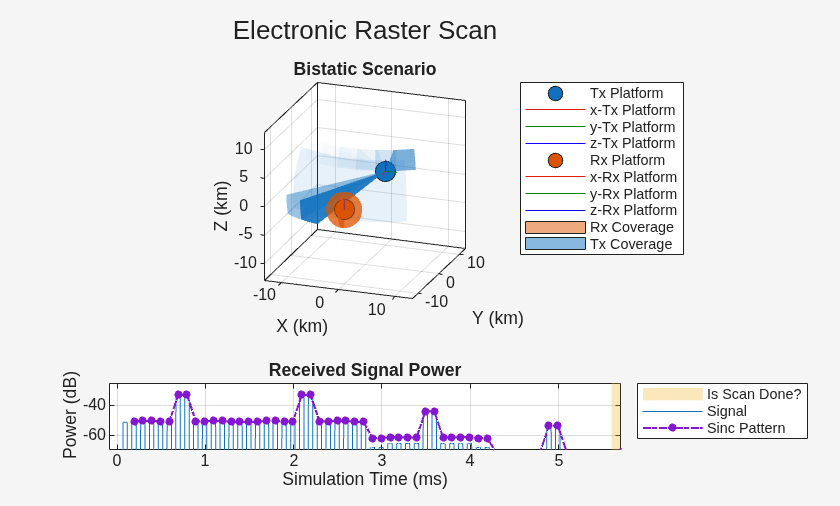
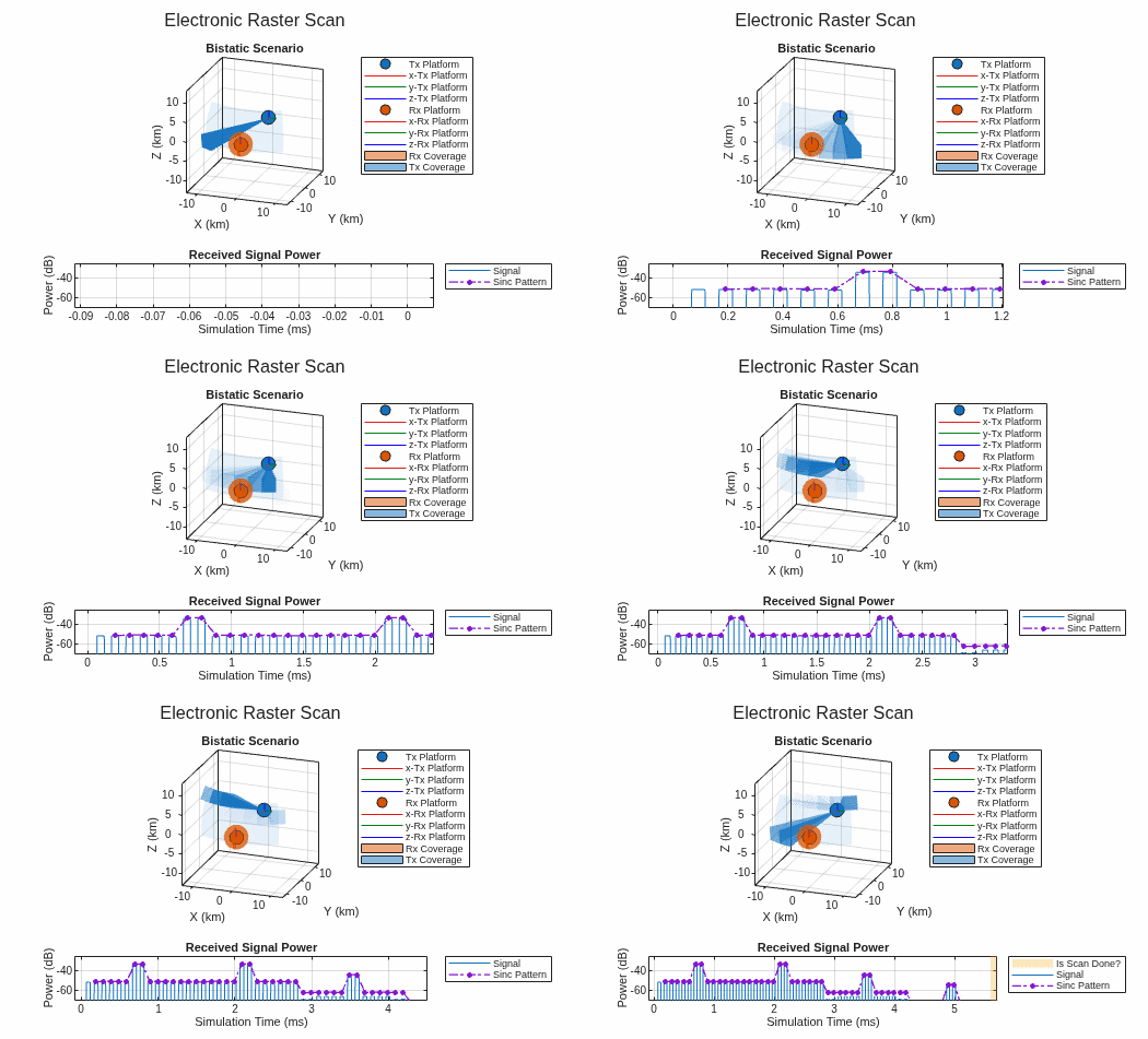
The received signal power peaks during the raster bar whose elevation coincides with the receive antenna. The sidelobe structure of the sinc antenna pattern is visible in the weaker returns from adjacent bars. Unlike the mechanical raster, which reverses direction at the end of each bar, the electronic raster always scans in the same direction along the primary axis because the beam repositions instantaneously.

Summary

This example demonstrated how to use radarScanController to simulate surveillance scan patterns for both mechanical and electronic scanners. Key differences between the two scan modes:

Mechanical scanners sweep continuously at a constant angular rate. They support return and reverse reset modes with configurable return durations, and their raster patterns reverse direction at the end of each bar.
Electronic scanners dwell at discrete angular positions for a fixed time before jumping instantaneously to the next. They have no return duration, and their raster patterns always scan in the same direction along the primary axis.

Both scanner types support sector and raster patterns with configurable scan limits, scan directions, 360-degree wrapping, and stationary modes. Use coverageConfig with theaterPlot to visualize beam coverage during simulation.

Local Helper Functions

function patdB = helperSincPattern(ang,bw)
% Sinc antenna element pattern
k3dB = abs(fzero(@(x)sinc(x)-1/sqrt(2),0));
patdB = mag2db(all(cosd(ang)>=0) * ... % include front hemisphere only
    abs( sinc(k3dB*sind(ang(1))/sind(bw(1)/2))* ... % azimuth
    sinc(k3dB*sind(ang(2))/sind(bw(2)/2)) ...  % elevation
    ));
end

function [scnro,txPlat,rxPlat,tp,plotScnro] = helperCreateScenario()
% Creates radarScenario with bistatic transmit and receive platforms, and
% theaterPlot to plot and update scenario truth
scnro = radarScenario;
traj = kinematicTrajectory(Position=[0 10e3 0],Orientation=quaternion([-90 0 0],"eulerd","ZYX","frame"));
txPlat = platform(scnro,Trajectory=traj);

traj = kinematicTrajectory(Position=[0 -10e3 0],Orientation=quaternion([90 0 0],"eulerd","ZYX","frame"));
rxPlat = platform(scnro,Trajectory=traj);

fig = helperFindFigure("Bistatic Scenario");
clf(fig);
tl = tiledlayout(fig,"vertical");

ax = nexttile(tl,1,[2 1]);
tp = theaterPlot(Parent=ax,AxesUnits=["km" "km" "km"],XLimits=13e3*[-1 1],YLimits=13e3*[-1 1],ZLimits=13e3*[-1 1]);
title(ax,fig.Name);

pltrs.TheaterPlot = tp;

txPlatPlotter = helperPlatformOrientationPlot(pltrs.TheaterPlot,txPlat,DisplayName="Tx Platform",LocalAxesLength=2e3);
pltrs.TxPlatFcn = @()helperPlatformOrientationPlotter(txPlatPlotter,txPlat);

rxPlatPlotter = helperPlatformOrientationPlot(pltrs.TheaterPlot,rxPlat,DisplayName="Rx Platform",LocalAxesLength=2e3);
pltrs.RxPlatFcn = @()helperPlatformOrientationPlotter(rxPlatPlotter,rxPlat);

plotScnro = @(varargin)helperUpdateScenarioPlotters(pltrs,varargin{:});
plotScnro();
view(pltrs.TheaterPlot.Parent,20,20);
end

function platPlotter = helperPlatformOrientationPlot(tp,plat,varargin)
% Creates orientation plotter for a platform with colors based on platform ID
ax = tp.Parent;
[xdir,ydir,zdir] = deal(ax.XDir,ax.YDir,ax.ZDir);
clnup = onCleanup(@()set(ax,XDir=xdir,YDir=ydir,ZDir=zdir));
clrs = colororder(tp.Parent);
platPlotter = orientationPlotter(tp,"MarkerFaceColor",clrs(plat.PlatformID,:),"LocalAxesLength",1e3,varargin{:});
end

function helperPlatformOrientationPlotter(platPlotter,plat)
% Plotter for platform's orientation
plotOrientation(platPlotter,orientation(plat,"quaternion","cartesian"),position(plat,"cartesian"));
end

function helperUpdateScenarioPlotters(pltrs)
% Calls scenario plotters to update theater plot
pltrs.TxPlatFcn();
pltrs.RxPlatFcn();
end

function sigPltr = helperSignalPowerPlot(tl,tau,patFcn,varargin)
% Creates signal power plot and returns its plotter function
sigPltr = @(sig,info,ang,isDone)helperSignalPowerPlotter(tl,sig,info,ang,isDone,tau,patFcn,varargin{:});
end

function helperSignalPowerPlotter(tl,sig,info,ang,isDone,tau,patFcn,fname)
% Plotter for signal power plot. Plots received signal power and
% corresponding antenna pattern. Creates animated GIF of figure when
% filename is provided
makeAnimation = nargin>7;

persistent lastAng cnt frm

% Reset the counter used to name the animated GIF files
if tl.GridSize(1)<3
    cnt = 0;
end

% Get the axes for the received signal power tile
ax = nexttile(tl,3,[1 1]);

% Reset the axes
if info.StartTime==0
    cla(ax);
    legend(ax,"off");
end

if isempty(sig)
    return
end

% Compute the received signal sample times
len = size(sig,1);
tt = (0:len-1).'/info.SampleRate + info.StartTime;

% Update the received signal power plot. Create a new plot if one doesn't
% exist.
h = findall(ax,Type="line",DisplayName="Signal");
x = tt.'*1e3;
y = mag2db(abs(sig)).';
if any(ishghandle(h))
    set(h,XData=[h.XData x],YData=[h.YData y]);
else
    plot(ax,x,y,DisplayName="Signal");
end

% Update the time span to match the signal
xlim(ax,([0 tt(end)]-tau)*1e3);

% If the axes was reset, reset the labels
if info.StartTime==0
    title(ax,"Received Signal Power");
    xlabel(ax,"Simulation Time (ms)");
    ylabel(ax,"Power (dB)");
    grid(ax,"on"); grid(ax,"minor");
    ylim(ax,[-70 -25])
    hold(ax,"on");
    lastAng = NaN(1,2);
end

% Update the sinc pattern plot. Create a new plot if one doesn't exist. The
% sinc pattern needs to include a simulation lag of one step, which is why
% the previous angle is used. This is because the bistaticReceiver returns
% the signal that was transmitted and collected during the previous
% simulation step.
h = findall(ax,Type="line",DisplayName="Sinc Pattern");
x = (tt(1)+tau)*1e3;
y = patFcn(lastAng);
if any(ishghandle(h))
    set(h,XData=[h.XData x],YData=[h.YData y]);
    frm = frm+1;
else
    h = plot(ax,x,y,"-.o",LineWidth=1,MarkerSize=3,SeriesIndex=4,DisplayName="Sinc Pattern");
    h.MarkerFaceColor = h.Color;
    uistack(h,"top");
    legend(ax,"show",Location="northeastoutside");
    cnt = cnt+1;
    frm = 0;
end
lastAng = paddata(ang,[1 2]);

if isDone
    % Update the "Is Scan Done" region. Create a new one if one doesn't
    % exist.
    len = size(sig,1);
    tt = [0 len-1].'/info.SampleRate + info.StartTime;

    x = tt*1e3;
    y = ylim(ax);
    [y,x] = meshgrid(y,x);
    verts = [x(:) y(:)];
    faces = [1 2 4 3];

    h = findall(ax,Type="patch",DisplayName="Is Scan Done?");
    if any(ishghandle(h))
        set(h,Vertices=[h.Vertices;verts],Faces=[h.Faces;faces+size(h.Vertices,1)]);
    else
        clrs = colororder(ax);
        h = patch(ax,Vertices=verts,Faces=faces,FaceColor=clrs(3,:),FaceAlpha=0.3,EdgeColor="none",DisplayName="Is Scan Done?");
        uistack(h,"bottom");
    end
end

% Capture the animated GIFs used in the published example
if makeAnimation && mod(frm,3)==0 % capture every 3 frames
    im = print(ax.Parent.Parent,"-RGBImage","-r90");
    [A,map] = rgb2ind(im,64);

    fname = fname + "_" + cnt + ".gif";
    if exist(fname,"file")
        imwrite(A,map,fname,"gif",WriteMode="append",DelayTime=0.3);
    else
        imwrite(A,map,fname,"gif",WriteMode="overwrite",LoopCount=inf,DelayTime=0.3);
    end
end
end

function fig = helperFindFigure(name,args)
% Reuses figure with same name, creates a new one if none exists
arguments
    name (1,1) string
    args.Visible (1,1) string = "on"
    args.WindowStyle (1,1) string = ""
end
fig = findall(groot,Type="figure",Name=name);
if ~any(ishghandle(fig))
    fig = figure(Name=name);
    for f = string(fieldnames(args))'
        if args.(f)~=""
            fig.(f) = args.(f);
        end
    end
end
fig = fig(1);
end

function coverageHistoryFcn = helperCoverageHistoryPlot(covPltr,args)
% Create coverage history plotters from a coveragePlotter
arguments
    covPltr (1,1)
    args.HistDepth (1,1) {mustBeInteger,mustBeNonnegative} = 16
    args.HistAlpha (1,2) {mustBeGreaterThan(args.HistAlpha,0), mustBeLessThanOrEqual(args.HistAlpha,1)} = [0.7 eps];
end
tp = covPltr.ParentPlot;
pltrs = tp.Plotters;

tag = covPltr.Tag;
isHistPltr = startsWith({pltrs.Tag}',tag+"_history");
if any(isHistPltr)
    histPltrs = pltrs(isHistPltr);
    for m = 1:numel(histPltrs)
        clearData(histPltrs(m));
        delete(histPltrs(m));
    end
end

clr = colororder(tp.Parent);
clr = clr(covPltr.Plotter.Map,:);
alpha = covPltr.Alpha;
histPltrs = [];
for m = 1:args.HistDepth
    histPltrs = cat(1,histPltrs,coveragePlotter(tp, Tag=tag + "_history" + m, ...
        Color=clr,Alpha=[args.HistAlpha].^m .* alpha));
end

helperCoverageHistoryPlotter(histPltrs); % Reset history
coverageHistoryFcn = @(covCfg)helperCoverageHistoryPlotter(histPltrs,covCfg);
end

function helperCoverageHistoryPlotter(histPltrs,covCfg)
% Plotter for coverage history
persistent buffCfgs

if isempty(buffCfgs)
    buffCfgs = containers.Map;
end

tag = histPltrs(1).Tag;

if nargin>1
    histDepth = numel(histPltrs);
    if isKey(buffCfgs,tag)
        theseCfgs = buffCfgs(tag);
        theseCfgs = [covCfg;theseCfgs];
        theseCfgs = theseCfgs(1:min(numel(theseCfgs),histDepth));

        buffCfgs(tag) = theseCfgs;
    else
        buffCfgs(tag) = covCfg;
    end

    theseCfgs = buffCfgs(tag);
    for m = 1:numel(theseCfgs)
        thisPltr = histPltrs(m);
        thisCfg = theseCfgs(m);
        plotCoverage(thisPltr,thisCfg);
        if all(isnan(thisCfg.Position))
            clearData(thisPltr);
        end
    end
else
    % Reset history
    if isKey(buffCfgs,tag)
        remove(buffCfgs,tag);
    end
end
end

function [txPose,rxPose,tgtPoses] = helperPlatformTruth(scenario,txPlat,rxPlat)
% Returns transmit, receive, and target platform truth, combining both
% platform pose and platform profile information onto a common structure
if scenario.IsEarthCentered
    poses = platformPoses(scenario,"quaternion","CoordinateSystem","Cartesian");
else
    poses = platformPoses(scenario,"quaternion");
end
profiles = platformProfiles(scenario);

txPose = helperTruth(txPlat,poses,profiles);
rxPose = helperTruth(rxPlat,poses,profiles);

iTgts = find([poses.PlatformID]~=txPlat.PlatformID & [poses.PlatformID]~=rxPlat.PlatformID);
numTgts = numel(iTgts);
tgtPoses = repmat(txPose,numTgts,1);
for m = 1:numTgts
    thisTgt = scenario.Platforms{iTgts(m)};
    tgtPoses(m) = helperTruth(thisTgt,poses,profiles);
end
end

function truth = helperTruth(plat,poses,profiles)
% Combines platform pose and profile information onto a common truth
% structure
iFnd = find([poses.PlatformID]==plat.PlatformID,1);
truth = poses(iFnd);
iFnd = find([profiles.PlatformID]==plat.PlatformID,1);
for f = string(setdiff(fieldnames(profiles),fieldnames(poses)))'
    truth.(f) = profiles(iFnd).(f);
end
end