Simulated Land Scenes for Synthetic Aperture Radar Image Formation

Since R2022a

A synthetic aperture radar (SAR) system uses platform motion to mimic a longer aperture to improve cross-range resolution. SAR data is often collected using platforms such as aircraft, spacecraft, or vehicle. Due to the movement of the platform, the data returned from the reflections of targets appears unfocused, looking at times like random noise. In SAR systems, essential information resides in the amplitude and phase of the received data. Phase-dependent processing is critical to the formation of focused images.

In this example, you will simulate an L-band remote-sensing SAR system. The simulation includes generating IQ signals from a scenario containing three targets and a wooded-hills land surface. The returned data will be processed using the range migration focusing algorithm.

For more information on key SAR concepts, see the Stripmap Synthetic Aperture Radar (SAR) Image Formation example.

Generate Simulated Terrain

Generate and plot a random height map for the land surface. The height map will be representative of a hilly scene with peaks up to about 200 m. It is important to ensure that the terrain resolution is less than the resolution of the imaging system. Based on the configuration of the helper function, the resolution of the map will be a little more than 1 meter in the X dimension and about 1.6 in the Y dimension. To increase the resolution of the generated map, increase the number of iterations. The roughness factor is often set to a value of 2. Smaller values result in rougher terrain, and larger values result in smoother terrain.

% Initialize random number generator
rng(2021)

% Create terrain
xLimits         = [900 1200]; % x-axis limits of terrain (m)
yLimits         = [-200 200]; % y-axis limits of terrain (m)
roughnessFactor = 1.75;       % Roughness factor
initialHgt      = 0;          % Initial height (m)
initialPerturb  = 200;        % Overall height of map (m) 
numIter         = 8;          % Number of iterations
[x,y,A] = helperRandomTerrainGenerator(roughnessFactor,initialHgt, ....
    initialPerturb,xLimits(1),xLimits(2), ...
    yLimits(1),yLimits(2),numIter);
A(A < 0) = 0; % Fill-in areas below 0
xvec = x(1,:); 
yvec = y(:,1);
resMapX = mean(diff(xvec))

resMapX = 
1.1719

resMapY = mean(diff(yvec))

resMapY = 
1.5625

% Plot simulated terrain
helperPlotSimulatedTerrain(xvec,yvec,A)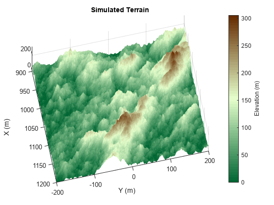

Figure contains an axes object. The axes object with title Simulated Terrain, xlabel X (m), ylabel Y (m) contains an object of type surface.

Specify the SAR System and Scenario

Define an L-band SAR imaging system with a range resolution approximately equal to 5 m. This system is mounted on an airborne platform flying at an altitude of 1000 meters. Verify the range resolution is as expected using the bw2rangeres function.

% Define key radar parameters
freq = 1e9;                        % Carrier frequency (Hz)
[lambda,c] = freq2wavelen(freq);   % Wavelength (m) 
bw = 30e6;                         % Signal bandwidth (Hz)
fs = 60e6;                         % Sampling frequency (Hz)
tpd = 3e-6;                        % Pulse width (sec) 

% Verify that the range resolution is as expected
rngRes = bw2rangeres(bw)

rngRes = 
4.9965

Specify the antenna aperture as 6 meters. Set the squint angle to 0 degrees for broadside operation.

% Antenna properties
apertureLength = 6;                % Aperture length (m) 
sqa = 0;                           % Squint angle (deg)

Set the platform velocity to 100 m/s and configure the platform geometry. The synthetic aperture length is 100 m as calculated by sarlen.

% Platform properties
v = 100;                           % Speed of the platform (m/s) 
dur = 1;                           % Duration of flight (s) 
rdrhgt = 1000;                     % Height of platform (m) 
rdrpos1 = [0 0 rdrhgt];            % Start position of the radar (m)
rdrvel = [0 v 0];                  % Radar plaform velocity
rdrpos2 = rdrvel*dur + rdrpos1;    % End position of the radar (m)
len = sarlen(v,dur)                % Synthetic aperture length (m)

len = 
100

Define the targets. The targets in this example are stationary and are intended to represent calibration targets. Set the target heights to 110 meters, relative to the surface. This height was selected such that targets may be occluded due to the hilly terrain.

% Configure the target platforms in x and y
targetpos = [1000,len/2,0;1020,len/2,0;1040,len/2,0]; % Target positions (m)
tgthgts = 110*ones(1,3); % Target height (m)
for it = 1:3 
    % Set target height relative to terrain
    [~,idxX] = min(abs(targetpos(it,1) - xvec)); 
    [~,idxY] = min(abs(targetpos(it,2) - yvec)); 
    tgthgts(it) = tgthgts(it) + A(idxX,idxY); 
    targetpos(it,3) = tgthgts(it); 
end

Next, set the reference slant range, which is used in subsequent processing steps such as determining appropriate pointing angles for the radar antenna. Calculate the cross-range resolutions using the sarazres function. Based on the geometry and radar settings, the cross-range resolution is about 2 meters.

% Set the reference slant range for the cross-range processing
rc = sqrt((rdrhgt - mean(tgthgts))^2 + (mean(targetpos(:,1)))^2);

% Antenna orientation
depang = depressionang(rdrhgt,rc,'Flat','TargetHeight',mean(tgthgts)); % Depression angle (deg)
grazang = depang; % Grazing angle (deg)

% Azimuth resolution
azResolution = sarazres(rc,lambda,len)  % Cross-range resolution (m)

azResolution = 
1.9572

Then, determine an appropriate pulse repetition frequency (PRF) for the SAR system. In a SAR system, the PRF has dual implications. The PRF not only determines the maximum unambiguous range but also serves as the sampling frequency in the cross-range direction. If the PRF is too low, the pulses are long in duration, resulting in fewer pulses illuminating a particular region. If the PRF is too high, the cross-range sampling is achieved but at the cost of reduced maximum range. The sarprfbounds function suggests maximum and minimum PRF bounds.

% Determine PRF bounds 
[swlen,swwidth] = aperture2swath(rc,lambda,apertureLength,grazang);
[prfmin,prfmax] = sarprfbounds(v,azResolution,swlen,grazang)

prfmin = 
51.0925

prfmax = 
6.4742e+05

For this example, set the PRF to 500 Hz.

% Select a PRF within the PRF bounds
prf = 500; % Pulse repetition frequency (Hz)

Now that the parameters for the radar and targets are defined. Set up a radar scene using radarScenario. Add the radar platform and targets to the scene with platform. Set the target radar cross section (RCS) to 5 dBsm, and plot the scene.

% Create a radar scenario
scene = radarScenario('UpdateRate',prf,'IsEarthCentered',false,'StopTime',dur);

% Add platforms to the scene using the configurations previously defined 
rdrplat = platform(scene,'Trajectory',kinematicTrajectory('Position',rdrpos1,'Velocity',[0 v 0]));

% Add target platforms
rcs = rcsSignature('Pattern',5); 
for it = 1:3
    platform(scene,'Position',targetpos(it,:),'Signatures',{rcs});
end

% Plot ground truth
helperPlotGroundTruth(xvec,yvec,A,rdrpos1,rdrpos2,targetpos)

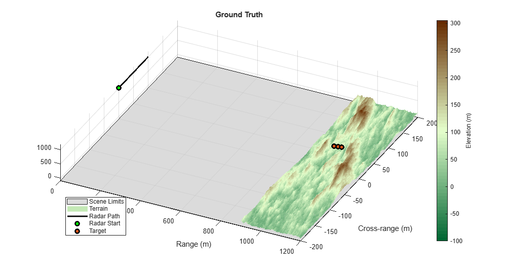
Figure contains an axes object. The axes object with title Ground Truth, xlabel Range (m), ylabel Cross-range (m) contains 5 objects of type surface, line. One or more of the lines displays its values using only markers These objects represent Scene Limits, Terrain, Radar Path, Radar Start, Target.

Note that the terrain generated has been limited in range and cross-range to the expected beam location. This is to conserve memory, as well as to speed up the simulation.

Define the Land Surface Reflectivity

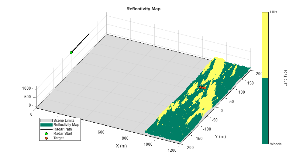
Now that the radar scenario and its platforms are set, define the land surface. First, select a reflectivity model. Radar Toolbox™ offers 7 different reflectivity models covering a wide range of frequencies, grazing angles, and land types. The asterisk denotes the default model. Type help landreflectivity or doc landreflectivity in the Command Window for more information on usage and applicable grazing angles for each model. The land reflectivity models are as follows.

APL: Mathematical model supporting low to high grazing angles over frequencies in the range from 1 to 100 GHz. Land types supported are urban, high-relief, and low-relief.
Barton*: Mathematical model supporting medium grazing angles over frequencies in the range from 1 to 10 GHz. Land types supported are rugged mountains, mountains, metropolitan, urban, wooded hills, rolling hills, woods, farm, desert, flatland, and smooth. This is the default model.
Billingsley: Empirical model valid for low grazing angles over frequencies from 3 MHz to 12 GHz. Land types supported are low-relief rural, low-relief forest, farm, desert, marsh, grassland, high-relief rural, high-relief forest, mountains, urban, low-relief urban.
GIT: Semi-empirical model for medium grazing angles over frequencies in the range from 3 to 15 GHz. Land types supported are soil, grass, tall grass, trees, and urban.
Morchin: Mathematical model for high grazing angles over frequencies in the range from 300 MHz to 8 GHz. Land types supported are desert, farm, woods, and mountains.
Nathanson: Empirical model for low to medium grazing angles over frequencies in the range from 1 to 36 GHz. Land types supported are desert, farm, woods, jungle, rolling hills, and urban.
Ulaby-Dobson: Semi-empirical model for low to medium grazing angles over frequencies in the range from 1 to 18 GHz. Land types supported are soil, grass, shrubs, and short vegetation.

For this example, use the default Barton model, since it has such a large number of land types. For terrain values above 100 meters, assign reflectivity values for wooded hills. Otherwise, set reflectivity values to woods. Plot the reflectivity map to see the assignments

% Specify custom reflectivity map
grazTable = 20:0.1:60;
freqTable = [1e9 10e9]; 
numSurfaces = 2;
reflectivityLayers = zeros(numel(grazTable),numel(freqTable),numSurfaces);
reflectivityLayers(:,:,1) = landreflectivity('Woods', ...
    grazTable,freqTable);
reflectivityLayers(:,:,2) = landreflectivity('WoodedHills', ...
    grazTable,freqTable);
reflectivityType = ones(size(A)); 
reflectivityType(A > 100) = 2; 

% Plot custom reflectivity map
helperPlotReflectivityMap(xvec,yvec,A,reflectivityType,rdrpos1,rdrpos2,targetpos)

Figure contains an axes object. The axes object with title Reflectivity Map, xlabel X (m), ylabel Y (m) contains 5 objects of type surface, line. One or more of the lines displays its values using only markers These objects represent Scene Limits, Reflectivity Map, Radar Path, Radar Start, Target.

Next, compose the custom reflectivity map for use by radarScenario using surfaceReflectivity. Set the Speckle property to Rayleigh. The surfaceReflectivity objects model speckle as an uncorrelated multiplicative factor as

$I = σ \cdot n$ ,

where $σ$ is the surface reflectivity and $n$ is an independent and identically distributed (IID) random value that is often defined as having unity mean noise. Common speckle models include Weibull, Rayleigh, and lognormal, which are all options provided by surfaceReflectivity. You can tailor the speckle with the distribution's corresponding properties. For a Rayleigh distribution, you can modify the SpeckleScale property.

reflectivityMap = surfaceReflectivity('Custom','Frequency',freqTable, ...
    'GrazingAngle',grazTable,'Reflectivity',reflectivityLayers, ...
    'Speckle','Rayleigh')

reflectivityMap = 
  surfaceReflectivityCustom with properties:

    EnablePolarization: 0
          Reflectivity: [401x2x2 double]
             Frequency: [1.0000e+09 1.0000e+10]
          GrazingAngle: [20 20.1000 20.2000 20.3000 20.4000 20.5000 20.6000 20.7000 20.8000 20.9000 21 21.1000 21.2000 21.3000 21.4000 21.5000 21.6000 21.7000 21.8000 21.9000 22 22.1000 22.2000 22.3000 22.4000 22.5000 22.6000 22.7000 ... ] (1x401 double)
               Speckle: 'Rayleigh'
          SpeckleScale: 0.7979

Add a land surface to the radar scenario using landSurface. Assign the random height map previously generated and the reflectivity map to the land surface.

% Add land surface to scene
s = landSurface(scene,'Terrain',A,'Boundary',[xLimits;yLimits], ...
    'RadarReflectivity',reflectivityMap, ...
    'ReflectivityMap',reflectivityType);

Configure the Radar Transceiver

In this section, configure the radar system properties. Define the antenna and the transmitted linear frequency modulated (LFM) waveform. Assign the radar sensor to the radar platform.

% Create a radar looking to the right
maxRange = 2500; % Maximum range for IQ collection
mountAngles = [0 depang 0];
rdr = radarTransceiver('MountingAngles',mountAngles,'NumRepetitions',1, ...
    'RangeLimits',[0 maxRange]);

% Set peak power
rdr.Transmitter.PeakPower = 50e3; 

% Set receiver sample rate and noise figure
rdr.Receiver.SampleRate = fs;
rdr.Receiver.NoiseFigure = 30; 

% Define transmit and receive antenna and corresponding parameters
antbw = ap2beamwidth(apertureLength,lambda); 
ant = phased.SincAntennaElement('FrequencyRange',[1e9 10e9],'Beamwidth',antbw);
rdr.TransmitAntenna.Sensor = ant;
rdr.TransmitAntenna.OperatingFrequency = freq;
rdr.ReceiveAntenna.Sensor = ant;
rdr.ReceiveAntenna.OperatingFrequency = freq;
antennaGain = aperture2gain(apertureLength^2,lambda); 
rdr.Transmitter.Gain = antennaGain;
rdr.Receiver.Gain = antennaGain;

% Configure the LFM signal of the radar
rdr.Waveform = phased.LinearFMWaveform('SampleRate',fs,'PulseWidth',tpd, ...
    'PRF',prf,'SweepBandwidth',bw); 

% Add radar to radar platform
rdrplat.Sensors = rdr;

Generate the Datacube

Now that the scene and the radar system are defined, generate returns from the land surface with the clutterGenerator method. By default, clutterGenerator will simulate clutter returns in the mainlobe. For more information about clutter modeling, see Introduction to Radar Scenario Clutter Simulation.

% Collect clutter returns with the clutterGenerator
clutterGenerator(scene,rdr,'Resolution',rngRes/2, ...
    'RangeLimit',maxRange);

% Initialize output IQ datacube
minSample = 500; % Minimum sample range
truncRngSamp = ceil(range2time(maxRange)*fs); % Limit the number of samples
T = 1/prf; % Pulse repetition interval (sec)
numPulses = dur/T + 1; % Number of pulses 
raw = zeros(numel(minSample:truncRngSamp),numPulses); % IQ datacube

Data is collected with the receive method. Either load in the data or simulate the raw SAR returns. If you choose to simulate the IQ, as the IQ data is received, a plot of the raw signal returns is generated. Otherwise, the unprocessed datacube is plotted at once. The raw signal is the collection of pulses transmitted in the cross-range direction. The plot shows the real part of the signal for the three targets and the land surface.

% Collect IQ 
ii = 1; 
hRaw = helperPlotRawIQ(raw,minSample);
simulateData = false; % Change to true to simulate IQ
if simulateData
    while advance(scene) %#ok<UNRCH>
        tmp = receive(scene); % nsamp x 1
        raw(:,ii) = tmp{1}(minSample:truncRngSamp);
        if mod(ii,100) == 0 % Update plot after 100 pulses
            helperUpdatePlotRawIQ(hRaw,raw);
        end
        ii = ii + 1;
    end
else
    load('rawSAR.mat');
end
helperUpdatePlotRawIQ(hRaw,raw);

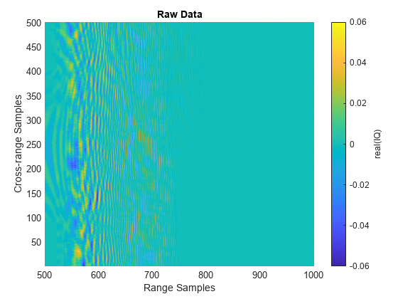
Figure contains an axes object. The axes object with title Raw Data, xlabel Range Samples, ylabel Cross-range Samples contains an object of type surface.

As is evident in the fully formed plot, the returns from the targets and the land surface are widely distributed in range and cross-range. Thus, it is difficult to distinguish the individual targets in the raw two-dimensional SAR data. The area where it is evident that returns are present is the mainlobe of the antenna. If you want to image a larger region, a couple of changes you can implement are:

Increase the altitude of the SAR imaging platform or
Increase the beamwidth.

Visualize SAR Data

Focus the image using the range migration algorithm. The range-migration algorithm corrects for the range-azimuth coupling, as well as the azimuth-frequency dependence. The algorithm proceeds as:

FFT: First, the algorithm performs a two-dimensional FFT. This transforms the SAR signal into wavenumber space.
Matched Filtering: Second, the algorithm focuses the image using a reference signal. This is a bulk focusing stage. The reference signal is computed for a selected range, often the mid-swath range. Targets at the selected range will be correctly focused, but targets away from the reference are only partially focused.
Stolt Interpolation: Next is a differential focusing stage that uses Stolt interpolation to focus the remainder of the targets.
IFFT: Finally, a two-dimensional IFFT is performed to return the data to the time domain.

Based on the radar waveform, use the rangeMigrationLFM function to form the single-look complex (SLC) image and plot the results. After range and cross-range processing, two targets can be distinguished from the background.

% Generating Single Look Complex image using range migration algorithm
slcimg = rangeMigrationLFM(raw,rdr.Waveform,freq,v,rc);
helperPlotSLC(slcimg,minSample,fs,v,prf,rdrpos1,targetpos, ...
    xvec,yvec,A)

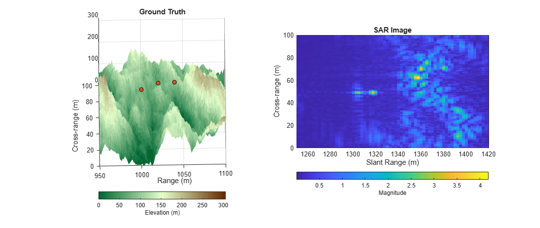
Figure contains 2 axes objects. Axes object 1 with title Ground Truth, xlabel Range (m), ylabel Cross-range (m) contains 2 objects of type surface, line. One or more of the lines displays its values using only markers Axes object 2 with title SAR Image, xlabel Slant Range (m), ylabel Cross-range (m) contains an object of type surface.

SAR images are similar to optical images, but the physics is quite different. Since SAR uses slant range to form images, higher elevation targets appear closer to the radar than lower elevation targets, resulting in higher elevation targets appearing at nearer ranges in the SAR image. This distortion is called layover and is noticeable in the image. Additionally, the actual grazing angles change slightly over the imaged swath, with shallower angles existing at farther ranges and steeper angles at closer ranges. These characteristics among others result in warped images in comparison to the Cartesian ground truth.

The occlusion method helps us to further interpret the results. Using the occlusion method on the land surface, determine the visibility of the targets throughout the scenario.

for it = 1:3
    % Determine whether the target was occluded
    occ = false(1,numPulses); 
    for ip = 1:numPulses
        rdrpos = rdrpos1 + rdrvel.*1/prf*(ip - 1); 
        occ(ip) = s.occlusion(rdrpos,targetpos(it,:));
    end

    % Translate occlusion values to a visibility status
    helperGetVisibilityStatus(it,occ)
end

Target 1 is not visible during the scenario (visible 0% of the data collection).
Target 2 is partially visible during the scenario (visible 84% of the data collection).
Target 3 is fully visible during the scenario (visible 100% of the data collection).

The first target is not visible at all, because it is occluded by the terrain. The second target is only partially visible throughout the collection. This causes missing data in the cross-range dimension, which results in the increased sidelobes and decreased signal power. The third target is fully visible throughout the target collection. It is bright and focused.

Summary

This example demonstrated how to generate IQ from a stripmap-based SAR scenario with three targets over land terrain. This example showed you how to:

Configure the SAR radar parameters,
Define the radar scenario,
Build a custom reflectivity map,
Add terrain to the scene with added speckle,
Generate IQ, and
Form a focused SAR image.

This example can be easily modified for other platform geometries, radar parameters, and surface types.

Supporting Functions

function [x,y,terrain] = helperRandomTerrainGenerator(f,initialHeight, ...
    initialPerturb,minX,maxX,minY,maxY,numIter)
%randTerrainGenerator Generate random terrain
% [x,y,terrain] = helperRandomTerrainGenerator(f,initialHeight, ...
%    initialPerturb,minX,maxX,minY,maxY,seaLevel,numIter)
%
% Inputs: 
%   - f                   = A roughness parameter.  A factor of 2 is a
%                           typical default. Lower values result in a 
%                           rougher terrain; higher values result in a 
%                           smoother surface.
%   - initialHeight       = Sets the initial height of the lattice before 
%                           the perturbations.
%   - initialPerturb      = Initial perturbation amount. This sets the 
%                           overall height of the landscape.
%   - minX,maxX,minY,maxY = Initial points. Provides some degree of control
%                           over the macro appearance of the landscape.
%   - numIter             = Number of iterations that affects the density 
%                           of the mesh that results from the iteration
%                           process.
%
% Output: 
%    - x                  = X-dimension mesh grid
%    - y                  = Y-dimension mesh grid
%    - terrain            = Two-dimensional array in which each value 
%                           represents the height of the terrain at that 
%                           point/mesh-cell

% Generate random terrain
dX = (maxX-minX)/2;
dY = (maxY-minY)/2;
[x,y] = meshgrid(minX:dX:maxX,minY:dY:maxY);
terrain = ones(3,3)*initialHeight;
perturb = initialPerturb;
for ii = 2:numIter
    perturb = perturb/f;
    oldX = x;
    oldY = y;
    dX = (maxX-minX)/2^ii;
    dY = (maxY-minY)/2^ii;
    [x,y] = meshgrid(minX:dX:maxX,minY:dY:maxY);
    terrain = griddata(oldX,oldY,terrain,x,y);
    terrain = terrain + perturb*randn(1+2^ii,1+2^ii);
    terrain(terrain < 0) = 0; 
end
end

function cmap = landColormap(n)
%landColormap Colormap for land surfaces
% cmap = landColormap(n)
%
% Inputs: 
%    - n     = Number of samples in colormap
%
% Output: 
%    - cmap  = n-by-3 colormap

c = hsv2rgb([5/12 1 0.4; 0.25 0.2 1; 5/72 1 0.4]);
cmap = zeros(n,3);
cmap(:,1) = interp1(1:3,c(:,1),linspace(1,3,n)); 
cmap(:,2) = interp1(1:3,c(:,2),linspace(1,3,n));
cmap(:,3) = interp1(1:3,c(:,3),linspace(1,3,n)); 
colormap(cmap);
end

function helperPlotSimulatedTerrain(xvec,yvec,A)
% Plot simulated terrain

figure()
hS = surf(xvec,yvec,A);
hS.EdgeColor = 'none';
hC = colorbar;
hC.Label.String = 'Elevation (m)';
landmap = landColormap(64);
colormap(landmap); 
xlabel('X (m)')
ylabel('Y (m)')
axis equal;
title('Simulated Terrain')
view([78 78])
drawnow
pause(0.25)
end

function helperPlotGroundTruth(xvec,yvec,A,rdrpos1,rdrpos2,targetpos)
% Plot ground truth

f = figure('Position',[505 443 997 535]);
movegui(f,'center');
% Plot boundary. Set plot boundary much lower than 0 for rendering reasons. 
hLim = surf([0 1200],[-200 200].',-100*ones(2),'FaceColor',[0.8 0.8 0.8],'FaceAlpha',0.7);
hold on;
hS = surf(xvec,yvec,A);
hS.EdgeColor = 'none';
hC = colorbar;
hC.Label.String = 'Elevation (m)';
landmap = landColormap(64);
colormap(landmap); 
hPlatPath = plot3([rdrpos1(1) rdrpos2(1)], ...
    [rdrpos1(2) rdrpos2(2)],[rdrpos1(3) rdrpos2(3)], ...
    '-k','LineWidth',2);
hPlatStart = plot3(rdrpos1(1),rdrpos1(2),rdrpos1(3), ...
    'o','LineWidth',2,'MarkerFaceColor','g','MarkerEdgeColor','k');
hTgt = plot3(targetpos(:,1),targetpos(:,2),targetpos(:,3), ...
    'o','LineWidth',2,'MarkerFaceColor',[0.8500 0.3250 0.0980], ...
    'MarkerEdgeColor','k');
view([26 75])
xlabel('Range (m)')
ylabel('Cross-range (m)')
title('Ground Truth')
axis tight;
zlim([-100 1200])
legend([hLim,hS,hPlatPath,hPlatStart,hTgt], ...
    {'Scene Limits','Terrain','Radar Path','Radar Start','Target'},'Location','SouthWest')
drawnow
pause(0.25)
end

function helperPlotReflectivityMap(xvec,yvec,A,reflectivityType,rdrpos1,rdrpos2,targetpos)
% Plot custom reflectivity map

f = figure('Position',[505 443 997 535]);
movegui(f,'center');
% Plot boundary. Set plot boundary much lower than 0 for rendering reasons. 
hLim = surf([0 1200],[-200 200].',-100*ones(2),'FaceColor',[0.8 0.8 0.8],'FaceAlpha',0.7);
hold on
hS = surf(xvec,yvec,A,reflectivityType);
hS.EdgeColor = 'none';
hold on;
colormap(summer(2));
hC = colorbar;
clim([1 2]); 
hC.Ticks = [1 2];
hC.TickLabels = {'Woods','Hills'};
hC.Label.String = 'Land Type';
hPlatPath = plot3([rdrpos1(1) rdrpos2(1)],[rdrpos1(2) rdrpos2(2)],[rdrpos1(3) rdrpos2(3)], ...
    '-k','LineWidth',2);
hPlatStart = plot3(rdrpos1(1),rdrpos1(2),rdrpos1(3), ...
    'o','MarkerFaceColor','g','MarkerEdgeColor','k');
hTgt = plot3(targetpos(:,1),targetpos(:,2),targetpos(:,3), ...
    'o','MarkerFaceColor',[0.8500 0.3250 0.0980],'MarkerEdgeColor','k');
view([26 75])
xlabel('X (m)')
ylabel('Y (m)')
title('Reflectivity Map')
axis tight; 
zlim([-100 1200])
legend([hLim,hS,hPlatPath,hPlatStart,hTgt], ...
    {'Scene Limits','Reflectivity Map','Radar Path','Radar Start','Target'},'Location','SouthWest')
drawnow
pause(0.25)
end

function hRaw = helperPlotRawIQ(raw,minSample)
% Plot real of raw SAR IQ 

figure()
[m,n] = size(raw); 
hRaw = pcolor(minSample:(m + minSample - 1),1:n,real(raw.'));
hRaw.EdgeColor = 'none';
title('Raw Data')
xlabel('Range Samples')
ylabel('Cross-range Samples')
hC = colorbar;
clim([-0.06 0.06])
hC.Label.String = 'real(IQ)'; 
drawnow
pause(0.25)
end

function helperUpdatePlotRawIQ(hRaw,raw)
% Update the raw SAR IQ plot

hRaw.CData = real(raw.'); 
clim([-0.06 0.06]);
drawnow
pause(0.25)
end

function helperPlotSLC(slcimg,minSample,fs,v,prf,rdrpos1,targetpos, ...
    xvec,yvec,A)
% Plot magnitude of focused SAR image alongside reflectivity map

% Cross-range y-vector (m)
numPulses = size(slcimg,2); 
du = v*1/prf; % Cross-range sample spacing (m) 
dky = 2*pi/(numPulses*du); % ku domain sample spacing (rad/m)
dy = 2*pi/(numPulses*dky); % y-domain sample spacing (rad/m)
y = dy*(0:(numPulses - 1)) + rdrpos1(2); % Cross-range y-vector (m) 

% Range vector (m)
c = physconst('LightSpeed'); 
numSamples = size(slcimg,1); 
samples = minSample:(numSamples + minSample - 1);
sampleTime = samples*1/fs; 
rngVec = time2range(sampleTime(1:end),c); 

% Initialize figure
f = figure('Position',[264 250 1411 535]);
movegui(f,'center')
tiledlayout(1,2,'TileSpacing','Compact');

% Ground Truth
nexttile;
hS = surf(xvec,yvec,A);
hS.EdgeColor = 'none';
hold on;
plot3(targetpos(:,1),targetpos(:,2),targetpos(:,3), ...
    'o','MarkerFaceColor',[0.8500 0.3250 0.0980],'MarkerEdgeColor','k');
landmap = landColormap(64);
colormap(landmap); 
hC = colorbar('southoutside');
hC.Label.String = 'Elevation (m)';
view([-1 75])
xlabel('Range (m)')
ylabel('Cross-range (m)')
title('Ground Truth')
axis equal
xlim([950 1100])
ylim([0 100])

% SAR Image
nexttile; 
slcimg = abs(slcimg).';
hProc = pcolor(rngVec,y,slcimg);
hProc.EdgeColor = 'none'; 
colormap(hProc.Parent,parula)
hC = colorbar('southoutside');
hC.Label.String = 'Magnitude';
xlabel('Slant Range (m)')
ylabel('Cross-range (m)')
title('SAR Image')
axis equal
xlim([1250 1420])
ylim([0 100])

drawnow
pause(0.25)
end

function helperGetVisibilityStatus(tgtNum,occ)
% Translate occlusion values to a visibility status

visibility = {'not','partially','fully'};
if all(occ)
    idx = 1;
elseif any(occ)
    idx = 2;
else
    idx = 3;
end
visString = visibility{idx};
pctCollect = sum(double(~occ))./numel(occ)*100;
fprintf('Target %d is %s visible during the scenario (visible %.0f%% of the data collection).\n', ...
    tgtNum,visString,pctCollect)
drawnow
pause(0.25)
end