Model-Based Policy Optimization (MBPO) Agent

Model-based policy optimization (MBPO) is a model-based, off-policy reinforcement learning algorithm for environments with a discrete or continuous action space. An MBPO agent contains an internal model of the environment, which it uses to generate additional experiences without interacting with the environment. Specifically, during training, the MBPO agent generates real experiences by interacting with the environment. These experiences are used to train the internal environment model, which is used to generate additional experiences. The training algorithm then uses both the real and generated experiences to update the agent policy. For more information on the different types of reinforcement learning agents, see Reinforcement Learning Agents.

In Reinforcement Learning Toolbox™, an MBPO agent is implemented by an rlMBPOAgent object.

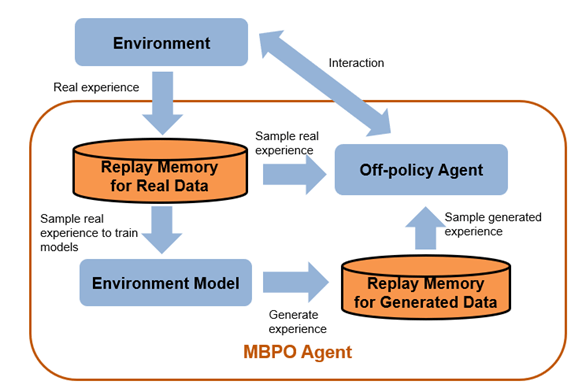
The following figure shows the components and behavior of an MBPO agent. The agent samples real experience data through environmental interaction and trains a model of the environment using this experience. Then, the agent updates the policy learnable parameters of its base agent using the real experience data and experience generated from the environment model.

Example of an MBPO agent interacting with an environment.

Note

MBPO agents do not support recurrent networks.

MBPO agents can be trained in environments with the following observation and action spaces.

Observation Space	Action Space
Continuous	Discrete or continuous

You can use the following off-policy agents as the base agent in an MBPO agent.

Action Space	Base Off-Policy Agent
Discrete	DQN agent — Deep Q-Network (DQN) Agent SAC agent with a discrete action space — Soft Actor-Critic (SAC) Agent
Continuous	DDPG agent — Deep Deterministic Policy Gradient (DDPG) Agent TD3 agent — Twin-Delayed Deep Deterministic (TD3) Policy Gradient Agent SAC agent with a continuous action space — Soft Actor-Critic (SAC) Agent

Note

Soft actor-critic agents with an hybrid action space cannot be used to build model based agents.

MBPO agents use an environment model that you define using an rlNeuralNetworkEnvironment object, which contains the following components. In general, these components use a deep neural network to learn the environment behavior during training.

One or more transition functions that predict the next observation based on the current observation and action. You can define deterministic transition functions using rlContinuousDeterministicTransitionFunction objects or stochastic transition functions using rlContinuousGaussianTransitionFunction objects.
A reward function that predicts the reward from the environment based on a combination of the current observation, current action, and next observation. You can define a deterministic reward function using an rlContinuousDeterministicRewardFunction object or a stochastic reward function using an rlContinuousGaussianRewardFunction object. You can also define a known reward function using a custom function.
An is-done function that predicts the termination signal based on a combination of the current observation, current action, and next observation. You can also define a known termination signal using a custom function.

During training, an MBPO agent:

Updates the environment model at the beginning of each episode by training the transition functions, reward function, and is-done function
Generates samples using the trained environment model and stores the samples in a circular experience buffer
Stores real samples from the interaction between the agent and the environment using a separate circular experience buffer within the base agent
Updates the actor and critic of the base agent using a mini-batch of experiences randomly sampled from both the generated experience buffer and the real experience buffer

Training Algorithm

MBPO agents use the following training algorithm, in which they periodically update the environment model and the base off-policy agent. To configure the training algorithm, specify options using an rlMBPOAgentOptions object.

Initialize the actor and critics of the base agent.
Initialize the transition functions, reward function, and is-done function in the environment model.
At the beginning of each training episode:
1. For each model-training epoch, perform the following steps. To specify the number of epochs, use the NumEpochForTrainingModel option.
  1. Train the transition functions. If the corresponding LearnRate optimizer option is 0, skip this step.
    Use a half-mean loss for an rlContinuousDeterministicTransitionFunction object and a maximum likelihood loss for an rlContinuousStochasticTransitionFunction object.
    To make each observation channel equally important, first compute the loss for each observation channel. Then, divide each loss by the number of elements in its corresponding observation specification.
    $L o s s = \sum_{i = 1}^{N_{o}} \frac{1}{M_{o i}} L o s s_{o i}$
    For example, if the observation specification for the environment is defined by [rlNumericSpec([10.1]) rlNumericSpec([4,1])], then N_o is 2, M_o₁ is 10, and M_o₂ is 4.
  2. Train the reward function. If the corresponding LearnRate optimizer option is 0 or a ground-truth custom reward function is defined, skip this step.
    Use a half-mean loss for an rlContinuousDeterministicRewardFunction object and a maximum likelihood loss for an rlContinuousStochasticRewardFunction object.
  3. Train the is-done function. If the corresponding LearnRate optimizer option is 0 or a ground-truth custom is-done function is defined, skip this step.
    Use a weighted cross-entropy loss function. In general, the terminal conditions (isdone = 1) occur much less frequently than nonterminal conditions (isdone = 0). To deal with the heavily imbalanced data, use the following weights and loss function.
    $\begin{array}{l} w_{0} = \frac{1}{\sum_{i = 1}^{M} (1 - T_{i})}, w_{1} = \frac{1}{\sum_{i = 1}^{M} T_{i}} \\ L o s s = \frac{- 1}{M} \sum_{i = 1}^{M} (w_{0} T_{i} \ln Y_{i} + w_{1} (1 - T_{i}) \ln (1 - Y_{i})) \end{array}$
    Here, M is the mini-batch size, T_i is a target, and Y_i is the output from the reward network for the ith sample in the batch. T_i = 1 when isdone is 1 and T_i = 0 when isdone is 0.
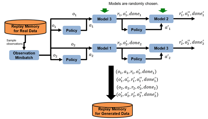
2. Generate samples using the trained environment model. The following figure shows an example of two roll-out trajectories with a horizon of two.
  1. Increase the horizon based on the horizon update settings defined in the ModelRolloutOptions object.
  2. Randomly sample a batch of N_R observations from the real experience buffer. To specify N_R, use the ModelRolloutOptions.NumRollout option.
  3. For each horizon step:
    Randomly divide the observations into N_M groups, where N_M is the number of transition models, and assign each group to a transition model.
    For each observation o_i, generate an action a_i using the exploration policy defined by the ModelRolloutOptions.NoiseOptions object. If ModelRolloutOptions.NoiseOptions is empty, use the exploration policy of the base agent.
    For each observation-action pair, predict the next observation o'₂ using the corresponding transition model.
    Using the environment model reward function, predict the reward value r_i based on the observation, action, and next observation.
    Using the environment model is-done function, predict the termination signal done_i based on the observation, action, and next observation.
    Add the experience (o_i,a_i,r_i,o'_i,done_i) to the generated experience buffer.
    For the next horizon step, substitute each observation with the predicted next observation.
For each step in each training episode:
1. Sample a mini-batch of M total experiences from the real experience buffer and the generated experience buffer. To specify M, use the MiniBatchSize option.
  - Sample N_real = ⌈M·R⌉ samples from the real experience buffer. To specify R, use the RealRatio option.
  - N_model = M – N_real samples from the generated experience buffer.
2. Train the base agent using the sampled mini-batch of data by following the update rule of the base agent. For more information, see the corresponding SAC, TD3, DDPG, or DQN training algorithm.

Tips

MBPO agents can be more sample-efficient than model-free agents because the model can generate large sets of diverse experiences. However, MBPO agents require much more computational time than model-free agents, because they must train the environment model and generate samples in addition to training the base agent.
To overcome modeling uncertainty, best practice is to use multiple environment transition models.
If they are available, it is best to use known ground-truth reward and is-done functions.
It is better to generate a large number of trajectories (thousands or tens of thousands). Doing so generates many samples, which reduces the likelihood of selecting the same sample multiple times in a training episode.
Since modeling errors can accumulate, it is better to use a shorter horizon when generating samples. A shorter horizon is usually enough to generate diverse experiences.
In general, an agent created using rlMBPOAgent is not suitable for environments with image observations.
When using a SAC base agent, taking more gradient steps (defined by the NumGradientStepsPerUpdate SAC agent option) makes the MBPO agent more sample-efficient. However, doing so increases the computational time.

The MBPO implementation in rlMBPOAgent is based on the algorithm in the original MBPO paper [1] but with the differences shown in the following table.

Original Paper	`rlMBPOAgent`
Generates samples at each environment step	Generates samples at the beginning of each training episode
Trains actor and critic using only generated samples	Trains actor and critic using both real data and generated data
Uses stochastic environment models	Uses either stochastic or deterministic environment models
Uses SAC agents	Can use SAC, DQN, DDPG, and TD3 agents

References

[1] Janner, Michael, Justin Fu, Marvin Zhang, and Sergey Levine. “When to Trust Your Model: Model-Based Policy Optimization.” In Proceedings of the 33rd International Conference on Neural Information Processing Systems, 12519–30. 1122. Red Hook, NY, USA: Curran Associates Inc., 2019.