Train a Robust Temperature Control Policy Using Vectorized Environments

R2026b

This example shows how to train a PPO agent using vectorized environments in MATLAB®. The heat pump environment changes the thermal properties and weather conditions across different environment instances. This allows you to train a policy that generalizes over a range of different dwellings and climates.

Define the Vectorized Environment

The environment for this example models a simple heat pump system that adds or removes heat from a dwelling. The environment changes the thermal properties of the dwelling and the weather conditions across instances to promote robust learning. The objective of the policy is to maintain the indoor temperature at a comfortable level while minimizing costs by controlling the heat pump throttle command.

The following equation describes the action input to the system:

$u_{k + 1} = c l i p (u_{k} + a_{k}, - 1, 1)$ , where:

$a_{k}$ is the scalar action signal that represents the change in throttle input commands between time steps.
$u_{k}$ is the heat pump throttle input.
- When $u_{k}$ > 0, the heat pump moves heat into the dwelling.
- When $u_{k}$ < 0, the heat pump moves heat out of the dwelling.

The following equation describes the system dynamics:

$T_{k + 1} = T_{k} + Δ t (\frac{{T o u t}_{k} - T_{k}}{R C} + \frac{M}{C} u_{k + 1})$ ,

where:

$T_{k}$ is the indoor temperature.
$Δ t$ is the 15-minute sample time.
${T o u t}_{k}$ is the outside temperature.
- The outside temperature is modeled by a noisy, asymmetric sine wave that represents daily temperature fluctuations. The mean and amplitude of the sine wave are also uniformly distributed to represent variations in seasonal conditions.
$R$ is the thermal resistance (°C/kW) of the structure.
- The environment reset function distributes $R$ uniformly between 1.5 and 9 °C/kW to represent dwellings with poor to good insulation.
$C$ is the thermal capacitance (kWh/°C) of the structure.
- The environment reset function distributes $C$ uniformly between 0.25 and 9 kWh/°C to represent dwellings with low to high thermal mass.
$M$ is the energy capacity of the heat pump.

The following equation describes the observation:

$s_{k + 1} = {[\begin{array}{cccc} {S T r}_{k - 2 : k + 1} & {S T o u t}_{k - 2 : k + 1} & {S T}_{k - 2 : k + 1} & u_{k - 2 : k + 1} \end{array}]}^{T}$ ,

where:

$S$ is a scaling factor that normalizes all temperature observations between 0 and 1.
${T r}_{k}$ is the target temperature.
$s_{k}$ is the normalized 16-element observation that contains the last 4 measured target temperatures, the outside temperatures, the indoor temperatures, and the heat pump throttle commands.
- Each observed measurement contains the last four samples. The sample history provides the temporal context that helps the agent to understand how the system responds over time. This temporal context enables the policy to infer uncertain, and unobserved, parameters such as $R$ and $C$ , during evaluation.

The following equations describe the reward function and the terminal condition:

$c o m f o r t = (T_{k + 1} > {T r}_{k + 1} - 1) & (T_{k + 1} < {T r}_{k + 1} + 1)$

$e n e r g y_c o s t = \frac{Δ t M g r i d_p r i c e}{μ} | u_{k + 1} |$

$r = 2 \cdot c o m f o r t - e n e r g y_c o s t - 0.5 a_{k}^{2}$

$d = (T_{k + 1} \geq 30) | (T_{k + 1} < 10)$ ,

where:

$r$ is the reward, which has 3 components:
- A bonus for the indoor temperature staying within 1°C of the target temperature.
- An operating cost of the heat pump. For this example, grid_price is 0.1348 $/kWh.
  - $μ$ is the coefficient of performance for the heat pump. For this example, $μ$ has a fixed value of 3.0.
- A penalty for large changes in heat pump throttle commands between samples.
$d$ is the terminal condition if the indoor temperature exceeds the too-cold (10°C) or too-hot (30°C) boundaries.

In this example, you use vectorization to implement the environment system of equations such that each column of a variable represents a separate environment instance. For example, T(:,i) is the indoor temperature of the ith environment instance. Expressing the environment variables in this way can greatly speed-up sample generation, leading to faster learning.

In this example, to create the vectorized environment for training the PPO agent, you provide a setup function, a reset function, and a step function as input arguments to rlFunctionVectorEnv.

View the Setup Function

The setup function allocates data to represent N environment instances. This function is called once the first time you that you simulate the vectorized environment and is called again only if you change the number of environment instances. The function takes as input an info structure that contains the number of environment instances to set up.

To set up data for N heat pump environments, the function allocates all variables that can vary across environment instances as arrays with N columns. Since the environment observation must contains 4-sample histories of the temperatures and the throttle commands, the setup functions allocates these observation variables as 4xN arrays.

Finally, the function includes all these variables into an env_data MATLAB structure, which is returned as the function output.

Display the setup function, which is provided with the example as a supporting file.

type heatpump_setup.m

function env_data = heatpump_setup(info)
% HEATPUMP_SETUP

% Copyright 2026 The MathWorks, Inc.

% Setup function for the vectorized heat pump environment.
% This function will allocate state and parameters for 
% each environment instance.

% Allocate thermal resistance (°C/kW) and capacitance (kWh/°C) for 
% each environment instance.
env_data.R              = zeros(1,info.NumEnv);
env_data.C              = zeros(1,info.NumEnv);

% Allocate data for the number of steps each environment
% instance takes along with characteristics of the 
% randomized weather model.
env_data.StepCount      = zeros(1,info.NumEnv,"uint32");
env_data.WeatherNoise   = zeros(1,info.NumEnv);
env_data.T_out_mean     = zeros(1,info.NumEnv);
env_data.T_out_amp      = zeros(1,info.NumEnv);

% Each environment instance will store measurements for 
% the last 4 outside temperatures, target temperatures,
% indoor temperatures, and the heat pump throttle command.
buff_size = 4;
env_data.T_out          = zeros(buff_size,info.NumEnv);
env_data.T_target       = zeros(buff_size,info.NumEnv);
env_data.T              = zeros(buff_size,info.NumEnv);
env_data.Throttle       = zeros(buff_size,info.NumEnv);

% Typical residential heat pumps have capacity vary
% from 2 to 16 kW power output
env_data.HeatPumpCapacity = 10.0;

% indoor min/max temperature bounds °C
env_data.T_bounds = [10.0,30.0];

% sample time for state integration in hours
env_data.Ts = 0.25;

% observation scaling factor
env_data.T_SCALE_FACTOR = 1/30;

View the Reset Function

The reset function defines how to reset the initial conditions and parameters of each environment instance at the start of each episode. The simulation or training function calls the reset function after any environment instance terminates, either due to a terminal condition or when the episode reaches the maximum number of allowed steps.

The reset function takes two input arguments; env_data, which is the MATLAB structure containing the environment state and parameter arrays, and resetidx, which is a logical array of the indices of the environments to reset. The function must output the "reset" observation buffer s along with the modified env_data data structure.

As described previously, the thermal resistance and capacitance of the dwelling are uniformly sampled during environment reset. Additionally, the initial indoor temperature, target temperature, and weather parameters are varied during environment reset. The reset function uses its local function usample to uniformly sample along the columns of these arrays.

When the states and parameters of the environment are reset, the observation buffer s is modified only for the environment indices that are reset.

Display the reset function, which is provided with the example as a supporting file.

type heatpump_reset.m

function [s,env_data] = heatpump_reset(env_data,resetidx)
% HEATPUMP_RESET

% Copyright 2026 The MathWorks, Inc.

% The reset function for the vectorized heat pump environment.
% This function will randomly reset states and parameters
% of each environment instance.

% Uniformly sample thermal resistance and capacitance
% values for each reset environment instance.
env_data.R  = usample(1.50,9.0,resetidx,env_data.R);
env_data.C  = usample(0.25,9.0,resetidx,env_data.C);

% Uniformly sample the target temperature and indoor 
% temperature initial condition.
env_data.T_target   = usample(18,24,resetidx,env_data.T_target);
env_data.T          = usample(15,27,resetidx,env_data.T       );

% Always have the heat pump throttle command start at 0.
env_data.Throttle(:,resetidx) = 0.0;

% Randomize the step count (start of day)
env_data.StepCount(1,resetidx) = randi(ceil(24./env_data.Ts) + 1,1,nnz(resetidx)) - 1;

% Uniformly sample the characteristics of the weather model.
env_data.T_out_mean = usample(5,15,resetidx,env_data.T_out_mean);
env_data.T_out_amp  = usample(2, 4,resetidx,env_data.T_out_amp );
env_data.WeatherNoise(1,resetidx) = 0.0;

% The initial outside temperature is consistent with the mean of the
% weather model.
env_data.T_out(:,resetidx) = repmat(env_data.T_out_mean(1,resetidx),size(env_data.T_out,1),1);

% Form the observations for only the reset environment
% instances.
s = {[
    env_data.T_SCALE_FACTOR.*env_data.T_out(:,resetidx);
    env_data.T_SCALE_FACTOR.*env_data.T_target(:,resetidx);
    env_data.T_SCALE_FACTOR.*env_data.T(:,resetidx);
    env_data.Throttle(:,resetidx);
    ]};

function x = usample(lower,upper,resetidx,x)
% Helper function to uniformly sample values
% in the range [lower,upper]. If x is buffered along the first
% dimension, the first row will be repeated for all rows.
n = nnz(resetidx); % evaluate the number of reset environments
x(:,resetidx) = lower + repmat((upper - lower).*rand(1,n,like=x),size(x,1),1);

View the Step Function

The step function defines how the environment advances from one time step to the next. It implements the equations described earlier, using vectorized MATLAB code.

The step function takes 2 input arguments; env_data, the MATLAB structure that contains the environment state and parameter arrays, and the action cell array a. The function must output the observations s, the rewards r, the is-done signal d, and the updated env_data structure that contains the new states of the system.

Display the step function, which is provided with the example as a supporting file.

type heatpump_step.m

function [s,r,d,env_data] = heatpump_step(env_data,a)
% HEATPUMP_STEP

% Copyright 2026 The MathWorks, Inc.

% The step function for the vectorized heat pump environment.
% This function will simulate the dynamics of each environment
% instance and generate the vectorized observation, reward,
% and isdone signals.

% Compute the time for each environment instance.
ts = env_data.Ts;
time = ts.*double(env_data.StepCount);

% Accumulate the change in heat pump throttle command
% from the action. The shiftbuff helper function is
% used to maintain a buffer of the last 4 values.
dthrottle = normclip(a{1}(:,:));
env_data.Throttle = shiftbuff(env_data.Throttle,...
    normclip(env_data.Throttle(end,:) + dthrottle));

% Compute the heat to be moved indoors.
q_heat_pump = env_data.Throttle(end,:).*env_data.HeatPumpCapacity;

% The basis of the weather model is an asymmetric sine wave,
% representing the warmest part of the day around 2PM.
daily_profile = sin(2.0.*pi.*(time - 8.0)./24.0);

% Add slow-changing weather noise unique for each
% environment instance using first-order filter.
weather_noise_std = 2.0;
a = 0.95;
b = weather_noise_std.*(1.0 - a);
env_data.WeatherNoise = a.*env_data.WeatherNoise + ...
    b.*randn(size(env_data.WeatherNoise),like=env_data.WeatherNoise);

% Compute the simulated outside temperature.
% The shiftbuff helper function is
% used to maintain a buffer of the last 4 values.
env_data.T_out = shiftbuff(env_data.T_out,...
    env_data.T_out_mean + env_data.T_out_amp.*daily_profile + ...
    env_data.WeatherNoise);

% Compute the thermal loss through the walls due
% to the temperature difference between indoors and outdoors.
q_walls = (env_data.T(end,:) - env_data.T_out(end,:))./env_data.R;

% Approximate the indoor temperature derivative using
% the first-order thermal dynamics model.
dTdt = (q_heat_pump - q_walls)./env_data.C;

% Integrate the temperature dynamics using forward Euler method.
% The shiftbuff helper function is
% used to maintain a buffer of the last 4 values.
env_data.T = shiftbuff(env_data.T,...
    env_data.T(end,:) + dTdt.*ts);

% Compute the cost for heating/cooling.
coeff_of_performance = 3.0;
grid_price = 0.1348; % $/kWh for Natick MA
energy_cost = ts.*grid_price.*abs(q_heat_pump)./coeff_of_performance;

% Compute if the indoor temperature is within the 
% the comfort band of +-1 °C of the target temperature.
t_upper = env_data.T_target(end,:) + 1.0;
t_lower = env_data.T_target(end,:) - 1.0;
comfortable = (env_data.T(end,:) >= t_lower) & (env_data.T(end,:) <= t_upper);

% Compute a penalty for large throttle changes between steps.
dthrottle_penalty = 1.0.*dthrottle.^2;

% Compute the reward.
r = 2.0.*double(comfortable) ...    % bonus for staying in the comfort region
    - energy_cost ...               % penalty for energy consumption
    - dthrottle_penalty;            % penalty for large throttle changes

% Terminate if indoor temperature is too hot or too cold.
d = uint8(...
    (env_data.T(end,:) < min(env_data.T_bounds)) | ...
    (env_data.T(end,:) > max(env_data.T_bounds)));

% update the step count
env_data.StepCount = env_data.StepCount + 1;

% Form the observations for all environment instances.
s = {[
    env_data.T_SCALE_FACTOR.*env_data.T_out;
    env_data.T_SCALE_FACTOR.*env_data.T_target;
    env_data.T_SCALE_FACTOR.*env_data.T;
    env_data.Throttle;
    ]};

function b = shiftbuff(b,u)
% Function to maintain a FIFO buffer along the 
% first dimension of the input buffer b. u_k will be inserted
% to the last row of b, u_k-1 will be moved to the second
% last row and so on. The first row is discarded upon insertion
% of u_k.

% transpose to shift along the 2nd dimension since MATLAB is 
% column major.
bt = b';
bt(:,1:(end-1)) = bt(:,2:end);
bt(:,end) = u(:);
% transpose back
b = bt';

function x = normclip(x)
% Helper function to clip element of x array between -1 and 1
x = max(min(x,1.0),-1.0);

Create the Vectorized Environment

To create the vectorized environment, pass the three required functions, the observation specifications, and the action specification as input arguments to rlFunctionVectorEnv.

num_obs = 16;
oinfo = rlNumericSpec([num_obs,1]);
ainfo = rlNumericSpec([      1,1]);
ainfo.UpperLimit =  1;
ainfo.LowerLimit = -1;

venv = rlFunctionVectorEnv(oinfo,ainfo,...
    @heatpump_step,...
    @heatpump_reset,...
    @heatpump_setup);

Specify Random Number Seed and Algorithm for Reproducibility

The example code might involve computation of random numbers at several stages. Fixing the random number stream seed at the beginning of some sections in the example code preserves the random number sequence in the section every time you run it, which is a necessary condition to reproduce the results. For more information, see Results Reproducibility.

Specify the random number stream with seed zero and random number algorithm Mersenne Twister. If your computer can use the GPU, also specify the GPU random number stream seed zero and random number algorithm Threefry. For more information on random number generation, see rng and gpurng (Parallel Computing Toolbox).

previousRngState = rng(0,"twister");
if canUseGPU(), previousGpuRngState = gpurng(0,"threefry"); end

The outputs previousRngState and previousGpuRngState are structures that contain information about the previous states of the stream. You will restore the state at the end of the example.

Define the Actor and Critic Models for the PPO Agent

Proximal Policy Optimization (PPO) Agent agents use a parameterized value function (critic) to estimate the value of observed states, and a stochastic policy (actor) to generate actions. Both the critic and the actor rely on multi-layer perceptron networks as internal approximation models. Each network contains three pairs of layers, and each pair consists of one fully-connected layer and one tanh layer.

Create the networks.

hlsz = 128;
common_layers = [
    featureInputLayer(num_obs,Name="obs")
    fullyConnectedLayer(hlsz)
    tanhLayer()
    fullyConnectedLayer(hlsz)
    tanhLayer()
    fullyConnectedLayer(hlsz)
    tanhLayer(Name="common_out")
    ];
critic_net = dlnetwork([ ...
    common_layers
    fullyConnectedLayer(1,Name="v")
    ]);
actor_net = dlnetwork([ ...
    common_layers
    fullyConnectedLayer(1,Name="a_mean_in")
    tanhLayer(Name="a_mean")
    ]);
actor_net = addLayers(actor_net,[ ...
    fullyConnectedLayer(1,Name="a_std_in")
    softplusLayer(Name="a_std") 
    ]);
actor_net = connectLayers(actor_net,"common_out","a_std_in");

Create the actor.

actor = rlContinuousGaussianActor(actor_net,oinfo,ainfo,...
    ActionMeanOutputNames="a_mean",...
    ActionStandardDeviationOutputNames="a_std");

Create the critic.

critic = rlValueFunction(critic_net,oinfo);

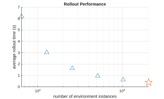
Determine the Optimal Number of Environment Instances for PPO Training

For this example, the PPO agent has a mini-batch size of 8192, and it collects 10 mini-batches before learning. Therefore, when you train the agent, the vectorized environment must generate 81920 samples per learning iteration.

To speed up training, tune the NumEnv property of the vectorized environment to the number of environment instances that generates 81920 samples in the least amount of time.

The upper bound on the number of environment instances is the largest number at which each instance still generates at least one full experience horizon of samples (that is, 32 samples) per learning iteration. For more information see the MiniBatchSize, ExperienceHorizon, and MaxMiniBatchPerEpoch properties of rlPPOAgentOptions.

ts                  = 0.25;             % sample time in hours
max_steps_per_ep    = ceil(1/ts)*24*4;  % 384 steps per episode: one episode = 4 days
mbsz                = 8192;             % mini-batch size
mb_per_epoch        = 10;               % number of mini-batches per epoch
exp_horizon         = ceil(8/ts);       % 32 samples horizon (covers 8 hours)
max_num_env         = floor(mbsz*mb_per_epoch/exp_horizon);

First, vary the number of environments with increment powers of 2.

num_envs = 2.^(6:floor(log2(max_num_env)));

Then, calculate the number of rollout steps needed to generate at least mbsz*max_mb_per_epoch samples.

rollout_steps = ceil(mbsz*mb_per_epoch./num_envs);

Run rollout multiple times to generate an average simulation time. For this example, run rollout three times for each value of NumEnv.

num_rollouts = 3;

Create a rlStochasticActorPolicy object to be able to simulate the environment against the policy.

policy = rlStochasticActorPolicy(actor);

To determine the optimal number of environment instances for training, run rollout to simulate the environment for each value of NumEnv.

n = numel(num_envs);
avg_duration = zeros(1,n);
for i = 1:n
    % Update NumEnv forces the setup function to be called again.
    venv.NumEnv = num_envs(i);
    tic;
    for j = 1:num_rollouts
        [~] = rollout(venv,policy,rollout_steps(i));
    end
    avg_duration(i) = toc/num_rollouts;
    fprintf("%u rollouts with %u environment instances took %g (s) on average\n",...
        num_rollouts,num_envs(i),avg_duration(i));
end

3 rollouts with 64 environment instances took 6.20536 (s) on average
3 rollouts with 128 environment instances took 3.04178 (s) on average
3 rollouts with 256 environment instances took 1.62725 (s) on average
3 rollouts with 512 environment instances took 0.955696 (s) on average
3 rollouts with 1024 environment instances took 0.615729 (s) on average
3 rollouts with 2048 environment instances took 0.384491 (s) on average

Determine which configuration took the least amount of time.

[min_duration,minidx] = min(avg_duration);
best_num_env = num_envs(minidx);

Plot the average rollout duration against the number of environment instances.

figure(1); cla;
hold("on");
plot(num_envs(num_envs ~= best_num_env), ...
    avg_duration(num_envs ~= best_num_env),...
    LineStyle   ="None",...
    Marker      ="^",...
    MarkerSize  =10);
plot(best_num_env,min_duration,...
    LineStyle   ="None",...
    Marker      ="pentagram",...
    MarkerSize  =20);
xscale("log");
xlabel("number of environment instances");
ylabel("average rollout time (s)");
title("Rollout Performance");
grid("on");
hold("off");

Figure contains an axes object. The axes object with title Rollout Performance, xlabel number of environment instances, ylabel average rollout time (s) contains 2 objects of type line. One or more of the lines displays its values using only markers

Set NumEnv to the number of environment instances that results the fastest simulation time.

venv.NumEnv = best_num_env;
fprintf("Selected %u environment instances for training\n",venv.NumEnv);

Selected 2048 environment instances for training

Create the PPO Agent

Specify the PPO agent hyperparameters.

aopt = rlPPOAgentOptions();
aopt.SampleTime                 = ts;
aopt.CriticOptimizerOptions     = rlOptimizerOptions( ...
    LearnRate=1e-3, ...
    GradientThreshold=0.5);
aopt.ActorOptimizerOptions      = rlOptimizerOptions( ...
    LearnRate=1e-3, ...
    GradientThreshold=0.5);
aopt.ExperienceHorizon          = exp_horizon;
aopt.EntropyLossWeight          = 0.01;
aopt.DiscountFactor             = 0.99;
aopt.GAEFactor                  = 0.95;
aopt.NumEpoch                   = 5;
aopt.MiniBatchSize              = mbsz;
aopt.LearningFrequency          = mbsz*mb_per_epoch; 
aopt.NormalizedAdvantageMethod  = "current";

Create the agent from the actor and critic objects.

agent = rlPPOAgent(actor,critic,aopt);

Configure the agent for GPU learning if a device is available.

agent.UseGPUForLearning = "auto";

Train the Agent

Set up the training options.

topts = rlTrainingOptions(...
    MaxEpisodes             =2.0e4,...
    MaxStepsPerEpisode      =max_steps_per_ep,...
    StopTrainingCriteria    ="none",...
    SaveAgentCriteria       ="none",...
    Verbose                 =false,...
    Plots                   ="none"); % Turn off plots for performance.

Create an Evaluator object that evaluates the policy after every 1000 episodes by running 15 episodes then averaging the cumulative rewards across the evaluation episodes.

evl = rlEvaluator(...
    EvaluationFrequency =1000,...
    NumEpisodes         =15,... 
    MaxStepsPerEpisode  =max_steps_per_ep);

Train the agent by using the train function. Training is computationally intensive and can take several minutes to complete. To save time while running this example, load a pretrained agent by setting doTraining to false. To train the agent yourself, set doTraining to true.

doTraining = false;
agentfile = "agent_data.mat";
if doTraining || ~isfile(agentfile)

    % Run the training.
    t_start = datetime("now");
    train_stats = train(agent,venv,topts,Evaluator=evl);
    t_end = datetime("now");
    train_time = t_end - t_start;

    % Save the agent.
    save(agentfile,"agent","train_stats","train_time");
else
    % Load the agent.
    load(agentfile,"agent","train_stats","train_time");
end

After training completes, or after you load the pretrained agent, plot the training progress.

episodes            = train_stats.EpisodeIndex;
cumulative_reward   = train_stats.EpisodeReward;
q0                  = train_stats.EpisodeQ0;
evaluation          = train_stats.EvaluationStatistic;
sample_throughput   = sum(train_stats.EpisodeSteps)/seconds(train_time);

figure(2); cla;
hold("on");
scatter(episodes,cumulative_reward,3 ,".");
scatter(episodes,q0               ,3 ,".");
scatter(episodes,evaluation       ,20,"*");
legend(["cumulative-reward","q0","evaluation"],Location="southeast");
xlabel("episode");
ylabel("cumulative reward");
title(sprintf("Training Progress (%0.2f minutes at %0.2fk samples/s)",...
    minutes(train_time),sample_throughput/1e3));
grid("on");
xscale("linear");
hold("off");

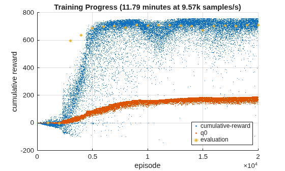
Figure contains an axes object. The axes object with title Training Progress (11.79 minutes at 9.57k samples/s), xlabel episode, ylabel cumulative reward contains 3 objects of type scatter. These objects represent cumulative-reward, q0, evaluation.

After 5000 episodes the training converges to a policy that achieves an average evaluation return above 700.

Validate the Policy in Simulink

Evaluate the performance of the trained policy by simulating it in a Simulink® model. Unlike the vectorized environment's discrete time dynamics, the model implements the heat transfer dynamics in continuous time, with the Policy block still operating in discrete time.

Open the model.

mdl = "rlHeatPump";
open_system(mdl);

To generate a Policy block, first, get the greedy policy from the PPO agent. Alternatively, you can get the exploration policy from the agent if you want to evaluate the stochastic policy instead.

policy = getGreedyPolicy(agent); % deterministic, greedy, policy
% policy = getExplorationPolicy(agent); % stochastic policy

Convert the policy sample time to seconds for use in the Simulink model.

policy.SampleTime = policy.SampleTime*3600;

Generate the policy block.

policyfile = "policy_data.mat";
if isfile(policyfile)
    delete(policyfile);
end
generatePolicyBlock(policy,MATFileName=policyfile);

For this example, since the model is already configured with a policy block in the Thermostat subsystem, close the generated model.

bdclose("untitled");

Next, to vary the workspace variables used by the model for each simulation, create a parameter grid for the thermal capacitance and resistance.

Create the parameter grid.

[C,R] = ndgrid([2 5 8],[2 5 8]);

Create Simulink.SimulationInput (Simulink) objects for each combination.

n = numel(R);
in(1:n) = Simulink.SimulationInput(mdl);
for i = 1:n
    % Start all simulations with an indoor temperature of 15 C
    % and the same random seed for weather noise generation.
    in(i) = setVariable(in(i),"T0"          ,15  );
    in(i) = setVariable(in(i),"noise_seed"  ,0   );
    in(i) = setVariable(in(i),"R"           ,R(i));
    in(i) = setVariable(in(i),"C"           ,C(i));
end

Simulate the model with for each combination.

out = sim(in,UseFastRestart="on",ShowProgress="off");

The model logs relevant signals. Plot the temperature response against the comfort zone boundaries for each scenario.

secs_to_hrs = 1/3600;
figure(3); cla();
hold("on");
for i = 1:n
    T = out(i).househeat_output.get("T").Values;
    stairs(T.Time*secs_to_hrs,T.Data,DisplayName=sprintf("T, R=%g, C=%g",R(i),C(i)));
end
Tout = out(1).househeat_output.get("Tout").Values;
stairs(Tout.Time*secs_to_hrs,Tout.Data,LineStyle="-.",DisplayName=sprintf("Tout"));
Tupper = out(1).househeat_output.get("Tupper").Values.Data;
Tlower = out(1).househeat_output.get("Tlower").Values.Data;
line([0,96],Tupper*[1 1],LineStyle="--",LineWidth=3,DisplayName="Tupper");
line([0,96],Tlower*[1 1],LineStyle="--",LineWidth=3,DisplayName="Tlower");

xlabel("time (hr)");
ylabel("Indoor Temperature (°C)");
title("Temperature Response");
legend(Location="eastoutside");
grid("on");
hold("off");

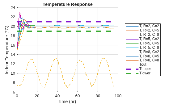
Figure contains an axes object. The axes object with title Temperature Response, xlabel time (hr), ylabel Indoor Temperature (°C) contains 12 objects of type stair, line. These objects represent T, R=2, C=2, T, R=2, C=5, T, R=2, C=8, T, R=5, C=2, T, R=5, C=5, T, R=5, C=8, T, R=8, C=2, T, R=8, C=5, T, R=8, C=8, Tout, Tupper, Tlower.

After a short warm-up period, the policy maintains the indoor temperature within the comfort bounds across all of the simulated scenarios.

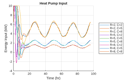
Plot the heat pump throttle command for each scenario.

figure(4); cla();
hold("on");
for i = 1:n
    u = out(i).househeat_output.get("throttle").Values;
    stairs(u.Time*secs_to_hrs,10*u.Data,DisplayName=sprintf("R=%g, C=%g",R(i),C(i)));
end

xlabel("Time (hr)");
ylabel("Energy Input (kW)");
title("Heat Pump Input");
legend(Location="eastoutside");
grid("on");
hold("off");

Figure contains an axes object. The axes object with title Heat Pump Input, xlabel Time (hr), ylabel Energy Input (kW) contains 9 objects of type stair. These objects represent R=2, C=2, R=2, C=5, R=2, C=8, R=5, C=2, R=5, C=5, R=5, C=8, R=8, C=2, R=8, C=5, R=8, C=8.

Plot the cost of operating the heat pump for each scenario.

figure(5); cla();
hold("on");
for i = 1:n
    cost = out(i).househeat_output.get("$").Values;
    stairs(cost.Time*secs_to_hrs,cost.Data,DisplayName=sprintf("R=%g, C=%g",R(i),C(i)));
end

xlabel("Time (hr)");
ylabel("Running Cost ($)");
title("Heat Pump Operation Cost");
legend(Location="eastoutside");
grid("on");
hold("off");

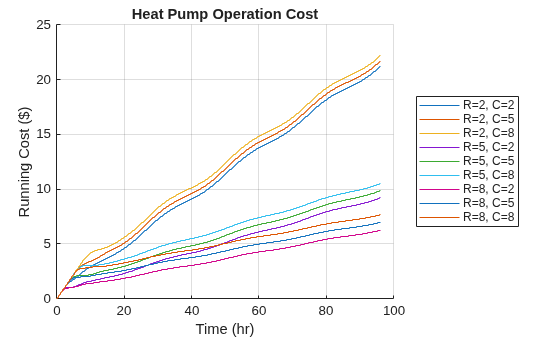
Figure contains an axes object. The axes object with title Heat Pump Operation Cost, xlabel Time (hr), ylabel Running Cost ($) contains 9 objects of type stair. These objects represent R=2, C=2, R=2, C=5, R=2, C=8, R=5, C=2, R=5, C=5, R=5, C=8, R=8, C=2, R=8, C=5, R=8, C=8.

These plots show that dwellings with higher thermal resistance require less energy to maintain a comfortable indoor temperature, resulting in lower operating costs.

Restore the random number stream using the information stored in previousRngState.

rng(previousRngState);
if canUseGPU(), gpurng(previousGpuRngState); end

Train a Robust Temperature Control Policy Using Vectorized Environments

Define the Vectorized Environment

View the Setup Function

View the Reset Function

View the Step Function

Create the Vectorized Environment

Specify Random Number Seed and Algorithm for Reproducibility

Define the Actor and Critic Models for the PPO Agent

Determine the Optimal Number of Environment Instances for PPO Training

Create the PPO Agent

Train the Agent

Validate the Policy in Simulink

See Also

Functions

Objects

Topics