Tune Hyperparameters Using Bayesian Optimization

This example uses:

This example shows how to tune reinforcement learning hyperparameters using Bayesian optimization. To train a reinforcement learning agent, you must specify the network architecture as well as the various hyperparameters for the agent's learning algorithm. Since the hyperparameter set may vary with applications, the default values may not be sufficient to learn the desired policy. You will use Bayesian optimization to tune a set of hyperparameters in this example.

Introduction

Bayesian optimization involves locating a point (a set of hyperparameters) that minimizes a real-valued function f(x), which is also known as the objective function.

In machine learning, hyperparameters are parameters that directly affect the learning process, whereas model parameters are directly affected by the learning process. In reinforcement learning, parameters such as the learning rates of the agent networks and minibatch sizes are hyperparameters. These parameters strongly affect the performance of the algorithm and it is often difficult and time-consuming to optimize them using techniques such as grid search or random search across the entire hyperparameter space. The Bayesian optimization algorithm can reduce the amount of evaluations needed to find the optimal hyperparameter set. The algorithm maintains a Gaussian process model of the objective function, and uses the objective function evaluations to iteratively train the model. The algorithm also uses an acquisition function to determine the next set of hyperparameters for evaluation. For more information see Bayesian Optimization Algorithm (Statistics and Machine Learning Toolbox).

In this example you will use the Optimize Cross-Validated Classifier Using bayesopt (Statistics and Machine Learning Toolbox) command to optimize hyperparameters. Using this command requires installation of the Statistics and Machine Learning Toolbox.

Create Environment Object

The environment is the lander vehicle environment from the Train PPO Agent for a Lander Vehicle example. The LanderVehicle class is provided in the example folder.

To view the environment code, open the LanderVehicle class.

open("LanderVehicle.m");

Create the environment object.

env = LanderVehicle()

env = 
  LanderVehicle with properties:

                Mass: 1
                  L1: 10
                  L2: 5
             Gravity: 9.8060
        ThrustLimits: [0 8.5000]
                  Ts: 0.1000
               State: [6x1 double]
          LastAction: [2x1 double]
         LastShaping: 0
    DistanceIntegral: 0
    VelocityIntegral: 0
           TimeCount: 0

Specify Variables To Optimize

You will optimize the hyperparameters of a proximal policy optimization (PPO) agent in this example. For running Bayesian optimization, specify the following hyperparameters using the optimizableVariable (Statistics and Machine Learning Toolbox) function. Also specify a search range for each hyperparameter.

Experience horizon for the PPO algorithm. A higher value can improve the stability of the training. Specify a range of 100 to 1000.
Mini-batch size for learning. Smaller mini-batches are computationally efficient but may introduce variance in training. Contrarily, larger batch sizes can make the training stable but require higher memory. Specify a range of 50 to 500.
Actor and critic learning rates. A large learning rate causes drastic updates which may lead to divergent behaviors, while a low value may require many updates before reaching the optimal point. Specify a range of 1e-6 to 1e-2.
Discount factor that controls the importance of long term rewards. Specify a range of 0.95 to 1.0.
Number of learning epochs. Specify a range of 1 to 10.
Clip factor for the PPO algorithm that limits the change in each policy update step. Specify a range of 0.01 to 0.1.
Entropy loss weight. A higher value promotes agent exploration. Specify the range of 0.01 to 0.1.

For more information on these parameters see rlPPOAgentOptions.

% size of minibatch
mbsz     = optimizableVariable( ...
    'MiniBatchSize', ...
    [50,500], ...
    'Type','integer');

% experience horizon
hrz      = optimizableVariable( ...
    'ExperienceHorizon', ...
    [100 600], ...
    'Type','integer');

% actor and critic learning rates
actorlr  = optimizableVariable('ActorLearnRate',[1e-6,1e-2]);
criticlr = optimizableVariable('CriticLearnRate',[1e-6,1e-2]);

% clip factor
clipf    = optimizableVariable('ClipFactor',[0.01,0.1]);

% entropy  loss weight
entw     = optimizableVariable('EntropyLossWeight',[0.01,0.1]);

% number of epochs
nepoch   = optimizableVariable('NumEpoch',[1,10],'Type','integer');

% discount factor
discf    = optimizableVariable('DiscountFactor',[0.95,1.0]);

Create an array of hyperparameters to optimize. This will be used for running the Bayesian optimization algorithm.

optimVars = [mbsz,hrz,actorlr,criticlr,clipf,entw,nepoch,discf];

Define Objective Function

The objective function runs one training of the agent using one set of hyperparameters and returns a score that represents the optimality of the hyperparameters. You can specify the cumulative reward obtained by the agent over an evaluation episode as the objective function value. Minimizing this score improves the performance of the agent. Alternately, you can also specify other metrics such as the best or last average episodic rewards as the objective function value.

The function performs the following steps:

Create the agent object using using networks having 400 units in their hidden layers.
Use the params input argument to configure the agent hyperparameters. params is a structure containing the hyperparameters configured in the previous section.
Train the agent for 3000 episodes, with at most 600 steps per episode.
Perform agent evaluations every 20 training episodes, with each evaluation running 5 simulations.
Return the objective (last evaluation score), constraints, and user data (trained agent and training result) as the function outputs.

Define the objective function.

function [objective,constraints,UserData] = objectiveFun(params,env)

% Fix the random stream for reproducibility
rng(0,"threefry");

% Get the observation and action input specifications
obsInfo = getObservationInfo(env);
actInfo = getActionInfo(env);

% Create initialization options for the agent networks, 
% specify the hidden unit size of 400
initOpts = rlAgentInitializationOptions(NumHiddenUnit=400);

% Create agent options and configure hyperparameters 
% using the params input argument
actorOpts  = rlOptimizerOptions( ...
    LearnRate=params.ActorLearnRate, ...
    GradientThreshold=1);
criticOpts = rlOptimizerOptions( ...
    LearnRate=params.CriticLearnRate, ...
    GradientThreshold=1);
agentOpts = rlPPOAgentOptions(...
    ExperienceHorizon      = params.ExperienceHorizon,...
    ClipFactor             = params.ClipFactor,...
    EntropyLossWeight      = params.EntropyLossWeight,...
    ActorOptimizerOptions  = actorOpts,...
    CriticOptimizerOptions = criticOpts,...
    MiniBatchSize          = params.MiniBatchSize,...
    NumEpoch               = params.NumEpoch,...
    SampleTime             = 0.1,...
    DiscountFactor         = params.DiscountFactor);

% Create the agent object
agent = rlPPOAgent(obsInfo,actInfo,initOpts,agentOpts);

% Training options
% Train the agent for a maximum of 3000 episodes, with 
% each episode lasting a maximum of 600 environment steps.
% To improve performance, do not store the simulation data 
% obtained from the episodes, and do not show the training plot.
trainOpts = rlTrainingOptions(...
    MaxEpisodes           = 3000,...
    MaxStepsPerEpisode    = 600,...
    StopTrainingCriteria  = "none",...
    SimulationStorageType = "none",...
    Plots                 = "none",...
    Verbose               = false);

% Agent evaluator
evl = rlEvaluator(EvaluationFrequency=20, NumEpisodes=5);

% Train the agent
result = train(agent, env, trainOpts, Evaluator=evl);

% Objective function score (last evaluation score)
score = result.EvaluationStatistic;
score(isnan(score)) = [];
objective = -score(end);

% Constraints (for this example there are no constraints)
constraints = [];

% Store the training result and trained agent in UserData
UserData.TrainingResult = result;
UserData.Agent = agent;

end

Run Bayesian Optimization

Fix the random stream for reproducibility. The output previousRngState is a structure that contains information about the previous state of the stream. You will restore the state at the end of the example.

previousRngState = rng(0,"twister")

previousRngState = struct with fields:
     Type: 'twister'
     Seed: 0
    State: [625x1 uint32]

Create an anonymous function handle for the objective function. This allows you to pass the environment object env to the objective function.

objFun = @(params) objectiveFun(params,env);

Tune the hyperparameters using the Optimize Cross-Validated Classifier Using bayesopt (Statistics and Machine Learning Toolbox) command.

Specify objFun and optimVars as input arguments.
Run the optimization using parallel workers. This requires the Parallel Computing Toolbox™ software. If you do not have the software installed, set UseParallel to false.
Since the optimization process is computationally intensive and takes several hours to complete, load a previously tuned result. If you want to run the optimization algorithm, set runOptimization to true.

runOptimization = false;
if runOptimization
    % run Bayesian optimization
    optimResults = bayesopt(objFun,optimVars,UseParallel=true);
else
    % load previously tuned result
    load("LanderOptimResults.mat","optimResults");
end

Analyze Results

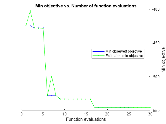
Plot the minimum observed and estimated function values versus the number of function evaluations.

plot(optimResults,@plotMinObjective)

Figure contains an axes object. The axes object with title Min objective vs. Number of function evaluations, xlabel Function evaluations, ylabel Min objective contains 2 objects of type line. These objects represent Min observed objective, Estimated min objective.

Get the best set of hyperparameters and best objective score using the bestPoint method. Store the iteration number for the best point in iteration.

[tunedParams,maxScore,iteration] = bestPoint(optimResults);

Display the maximum score and the iteration.

maxScore

maxScore = 
-541.7592

iteration

iteration = 
17

Display the related tuned parameters.

rows2vars(tunedParams)

ans=8×2 table
    OriginalVariableNames      Var1   
    _____________________    _________

    {'MiniBatchSize'    }          453
    {'ExperienceHorizon'}          853
    {'ActorLearnRate'   }    0.0021441
    {'CriticLearnRate'  }    0.0064594
    {'ClipFactor'       }     0.019635
    {'EntropyLossWeight'}     0.045334
    {'NumEpoch'         }            7
    {'DiscountFactor'   }      0.99282

Get the tuned agent and training result stored in the UserDataTrace property. For convenience, load the tuned agent and training result from disk.

if runOptimization
    % get the tuned agent and training result from the optimization
    userData    = optimResults.UserDataTrace{iteration};
    tunedAgent  = userData.Agent;
    tunedResult = userData.TrainingResult;
else
    % load previously tuned agent and training result
    load("LanderOptimResults.mat","tunedAgent","tunedResult");
end

View the training plot for the tuned agent.

show(tunedResult)

A snapshot of the training progress is shown below. You can expect different results due to randomness in training.

Simulate Tuned Agent

Fix the random stream for reproducibility.

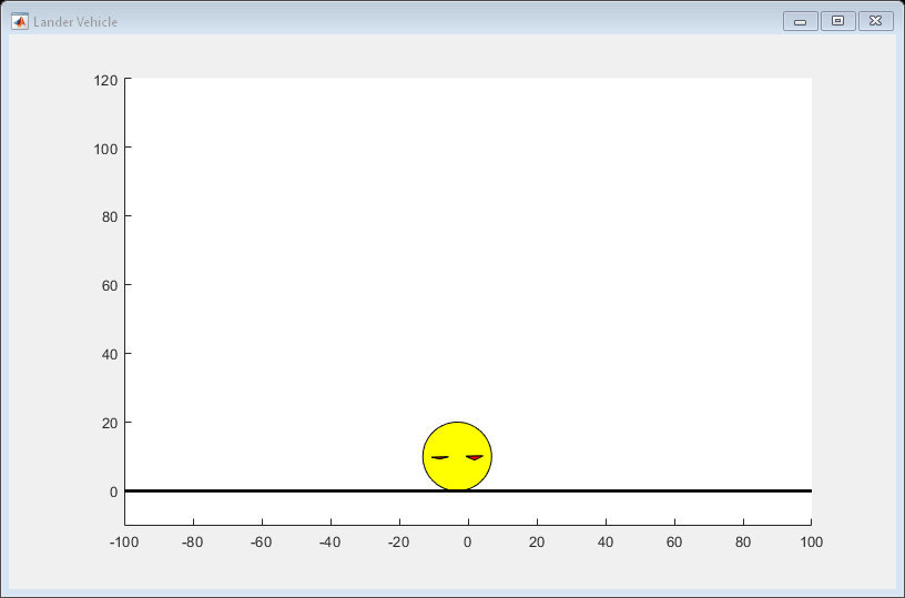
rng(0,"twister");

Plot the environment to see animation in a figure.

plot(env);

Simulate the tuned agent.

simOpts = rlSimulationOptions(MaxSteps=600);
experience = sim(tunedAgent,env,simOpts);

Figure Lander Vehicle contains an axes object. The axes object contains 7 objects of type rectangle, line, patch, text.

The lander vehicle is able to successfully land at the target location.

Display the total reward obtained from the simulation.

cumulativeReward = sum(experience.Reward.Data)

cumulativeReward = 
527.7665

Restore the random number stream using the information stored in previousRngState.

rng(previousRngState);

Related Examples

Log Training Data to Disk
Train PPO Agent for a Lander Vehicle
Optimize Cross-Validated Classifier Using bayesopt (Statistics and Machine Learning Toolbox)
Train Agent or Tune Environment Parameters Using Parameter Sweeping
Configure Exploration For Reinforcement Learning Agents

More About

Bayesian Optimization Algorithm (Statistics and Machine Learning Toolbox)
Train Reinforcement Learning Agents
Water Tank Reinforcement Learning Environment Model