Analyze Transmission Line

Open Live Script

This example shows you how to analyze a transmission line using RF Toolbox. The example analyzes a parallel plate transmission line, but you can also analyze other transmission line types using these steps.

The example:

First shows you how to analyze a transmission line in the frequency domain using an analytical model based on geometric properties.
Second it shows you how to create an equivalent representation of the transmission line model suitable for time domain simulation.
Finally the example shows you how to create a Verilog A module of the transmission line suitable for simulation in Spice-like circuit simulators.

Video Walkthrough

For a walkthrough of the example, play the video.

Build and Simulate Transmission Line

Create a txlineParallelPlate object to represent the transmission line, which is 0.1 meters long and 0.05 meters wide.

tline = txlineParallelPlate('LineLength',0.1,'Width',0.05);

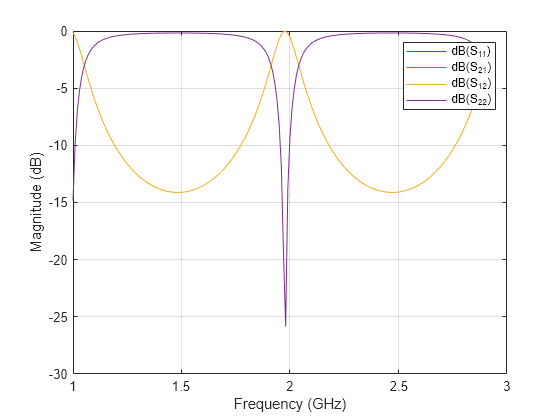
Define the range of frequencies over which to analyze S-parameters of the transmission line.

f = 1.0e9:1e7:2.9e9;
S = sparameters(tline,f);
rfplot(S);

$Figure contains an axes object. The axes object with xlabel Frequency (GHz), ylabel Magnitude (dB) contains 4 objects of type line. These objects represent dB(S_{11}), dB(S_{21}), dB(S_{12}), dB(S_{22}).$

Compute Transmission Line Transfer Function and Time-Domain Response

To compute the transfer function of the transmission line and its time-domain response, you must:

Calculate the Transfer Function
Fit and Validate the Transfer Function Model
Compute and Plot the Time-Domain Response

Calculate Transfer Function

Compute the transfer function from the frequency response data using the s2tf function. This function can be used to extract the TF from any arbitrary 2 port S-parameter data, for example from EM analysis or VNAs.

TrFunc = s2tf(S);

Fit and Validate Transfer Function Model

Fit a rational function to the computed data and store the result in an rfmodel object.

RationalFunc = rational(f,TrFunc)

RationalFunc = 
  rational with properties:

      NumPorts: 1
      NumPoles: 9
         Poles: [9x1 double]
      Residues: [1x1x9 double]
    DirectTerm: 0
         ErrDB: -74.1053

Compute the frequency response of the fitted model data.

[fresp] = freqresp(RationalFunc,f);

Plot the amplitude of the frequency response of the fitted model data and that of the computed or original data.

figure
plot(f/1e9,20*log10(abs(fresp)),'o-',f/1e9,20*log10(abs(TrFunc)))
xlabel('Frequency, GHz')
ylabel('Amplitude, dB')
legend('Fitted Model Data','Original Data')

Figure contains an axes object. The axes object with xlabel Frequency, GHz, ylabel Amplitude, dB contains 2 objects of type line. These objects represent Fitted Model Data, Original Data.

The amplitude of the model data is very close to the amplitude of the computed data. You can control the tradeoff between model accuracy and model complexity by specifying the optional tolerance argument, Tolerance, to the rational object, as described in Export Verilog-A Model.

Plot the phase angle of the frequency response of the fitted model data and that of the Original data:

figure
plot(f/1e9,unwrap(angle(fresp)),'o-',...
    f/1e9,unwrap(angle(TrFunc)))
xlabel('Frequency, GHz')
ylabel('Phase Angle, radians')
legend('Fitted Data','Original Data')

Figure contains an axes object. The axes object with xlabel Frequency, GHz, ylabel Phase Angle, radians contains 2 objects of type line. These objects represent Fitted Data, Original Data.

The phase angle of the model data is very close to the phase angle of the computed data.

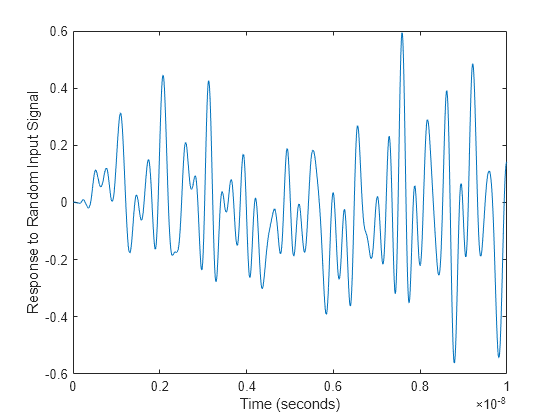
Compute and Plot Time-Domain Response

To compute and plot the time-domain response of the transmission line, first create a random input signal and compute the time response, tresp, of the fitted model data to the input signal:

SampleTime = 1e-12;
NumberOfSamples = 1e4;
OverSamplingFactor = 25;
InputTime = double((1:NumberOfSamples)')*SampleTime;
InputSignal = ...
    sign(randn(1, ceil(NumberOfSamples/OverSamplingFactor)));
InputSignal = repmat(InputSignal, [OverSamplingFactor, 1]);
InputSignal = InputSignal(:);

[tresp,t] = timeresp(RationalFunc,InputSignal,SampleTime);

Plot the time response of the fitted model data:

figure
plot(t,tresp)
xlabel('Time (seconds)')
ylabel('Response to Random Input Signal')

Figure contains an axes object. The axes object with xlabel Time (seconds), ylabel Response to Random Input Signal contains an object of type line.

Export Verilog-A Model

Export a Verilog-A model of the transmission line. You can use this model in other simulation tools for detailed time-domain analysis and system simulations.

Use the writeva function to write a Verilog-A module for RationalFunc to the file tline.va. The module has one input, tline_in, and one output, tline_out. The method returns a status of True, if the operation is successful, and False if it is unsuccessful.

status = writeva(RationalFunc,'tline','tline_in','tline_out')

status = logical
   1

For more information on the writeva method and its arguments, see the writeva reference page.