Superheterodyne Receiver Using RF Budget Analyzer App

Introduction

RF system designers begin the design process with a budget specification for how much gain, noise figure (NF), and nonlinearity (IP3) the entire system must satisfy. To assure the feasibility of an architecture modeled as a simple cascade of RF elements, designers calculate both the per-stage and cascade values of gain, noise figure, and third-order intercept point (IP3).

Using the RF Budget Analyzer app, you can:

For more information, see RF Budget Analyzer app.

Video Walkthrough

For a walkthrough of the example, play the video.

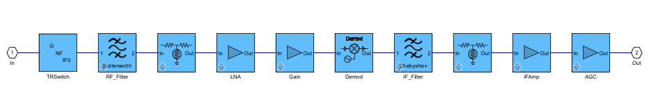
Build Superheterodyne Receiver

The first components in the superheterodyne receiver system architecture are the antenna and TR switch. You can replace the antenna element with the effective power reaching the switch.

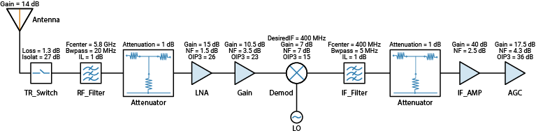
1. The receiver uses the TR switch to switch between the transmitter and the receiver. The switch adds a loss of 1.3 dB to the system. Use the rfelement object to create a TR switch with a gain of –1.3 dB, and output third-order intercept (OIP3) of 37 dBm. To match the RF budget results from reference [1], assume that the noise figure is 2.3 dB.

elements(1) = rfelement('Name','TRSwitch','Gain',-1.3,'NF',2.3,'OIP3',37);

2. Next element in the chain is the RF bandpass filter. Use an rffilter object to model an RF bandpass filter. For more information about the design specification of the RF Bandpass filter used in this example, see Design IF Butterworth Bandpass Filter.

Fcenter = 5.8e9;
Bwpass  = 20e6;
elements(2) = rffilter('ResponseType','Bandpass', ...
    'FilterType','Butterworth','FilterOrder',6, ...
    'PassbandAttenuation',10*log10(2), ...
    'Implementation','Transfer function', ...
    'PassbandFrequency',[Fcenter-Bwpass/2 Fcenter+Bwpass/2], ...
    'Name','RF_Filter');

3. The S-parameters for the element(2) filter are not ideal. Therefore, use a 1 dB attenuator to model the insertion loss of the filter into the system.

elements(3) = attenuator("Attenuation",1);

4. Use the amplifier object to model a Low Noise Amplifier block with a gain of 15 dB, noise figure of 1.5 dB, and OIP3 of 26 dBm.

elements(4) = amplifier('Name','LNA','Gain',15,'NF',1.5,'OIP3',26);

5. Model a Gain block with a gain of 10.5 dB, noise figure of 3.5 dB, and OIP3 of 23 dBm.

elements(5) = amplifier('Name','Gain','Gain',10.5,'NF',3.5,'OIP3',23);

6. The receiver downconverts the RF frequency to an IF frequency of 400 MHz. Use the modulator object to create a Demodulator block with local oscillator (LO) frequency of 5.4 GHz, gain of –7 dB, noise figure of 7 dB, and OIP3 of 15 dBm.

elements(6) = modulator('Name','Demod','Gain',-7,'NF',7,'OIP3',15,      ...
    'LO',5.4e9, 'ConverterType','Down');

7. Model an IF bandpass filter using rffilter object.

Fcenter = 400e6;
Bwpass  = 5e6;
elements(7) = rffilter('ResponseType','Bandpass', ...
    'FilterType','Chebyshev','FilterOrder',4, ...
    'PassbandAttenuation',0.1, ...
    'Implementation','Transfer function', ...
    'PassbandFrequency',[Fcenter-Bwpass/2 Fcenter+Bwpass/2], ...
    'Name','IF_Filter');

8. The S-parameters for the element(7) filter are not ideal. Therefore, use a 1 dB attenuator to model the insertion loss of the filter into the system.

elements(8) = attenuator("Attenuation",1);

9. Model an IF Amplifier block with a gain of 40 dB and a noise figure of 2.5 dB.

elements(9) = amplifier('Name','IFAmp','Gain',40,'NF',2.5);

10. As seen in the references, the receiver uses an Automatic Gain Control (AGC) block where the gain varies with the available input power. For an input power of –80 dB, the AGC gain is at a maximum of 17.5 dB. Use an Amplifier block to model an AGC. Model an AGC block with a gain of 17.5 dB, noise figure of 4.3 dB, and OIP3 of 36 dBm.

elements(10) = amplifier('Name','AGC','Gain',17.5,'NF',4.3,'OIP3',36);

Cascade all the elements to construct an RF chain. Use the rfbudget object to calculate the RF budget of the superheterodyne receiver. Set Input frequency to 5.8 GHz and signal bandwidth to 20 MHz. Replace the antenna element with the effective available input power which is estimated to be –66 dB when reaching the TR switch.

superhet = rfbudget('Elements',elements,'InputFrequency',5.8e9,  'AvailableInputPower',-66,'SignalBandwidth',20e6)

superhet = 
  rfbudget with properties:

               Elements: [1x10 rf.internal.rfbudget.Element]
         InputFrequency: 5.8 GHz
    AvailableInputPower: -66 dBm
        SignalBandwidth:  20 MHz
                 Solver: Friis      
             AutoUpdate: true

   Analysis Results
        OutputFrequency: (GHz) [  5.8    5.8    5.8    5.8      5.8     0.4     0.4     0.4     0.4    0.4]
            OutputPower: (dBm) [-67.3  -67.3  -68.3  -53.3    -42.8   -49.8   -49.9   -50.9   -10.9    6.6]
         TransducerGain: (dB)  [ -1.3   -1.3   -2.3   12.7     23.2    16.2    16.1    15.1    55.1   72.6]
                     NF: (dB)  [  2.3    2.3  3.112   4.39    4.494   4.524   4.524   4.534    4.57   4.57]
                   IIP2: (dBm) []                                                                          
                   OIP2: (dBm) []                                                                          
                   IIP3: (dBm) [ 38.3   38.3   38.3  13.29  -0.3904  -3.824  -3.824  -3.824  -3.824  -36.6]
                   OIP3: (dBm) [   37     37     36  25.99    22.81   12.38   12.28   11.28   51.28     36]
                    SNR: (dB)  [32.66  32.66  31.85  30.57    30.47   30.44   30.44   30.43   30.39  30.39]

View the analysis in the RF Budget Analyser app by typing this command at the command line. The app displays the cascade values such as output frequency of the receiver, output power, gain, noise figure, OIP3, and Signal-to- Noise-Ratio (SNR). The RF Budget Analyzer app saves the model in a MAT-file.

show(superhet);

Plot Cascade Transducer Gain and Cascade Noise Figure

Plot the cascade transducer gain of the receiver using the rfplot function. You can also use the Plot button on the RF Budget Analyzer app to plot the different output values.

rfplot(superhet,'GainT')
view(90,0)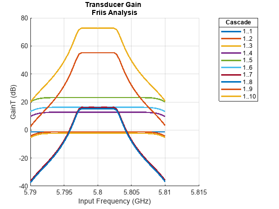

2. Plot the cascade noise figure of the receiver.

rfplot(superhet,'NF')
view(90,0)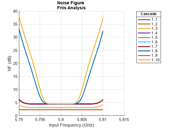

Export to MATLAB Script

Export the model to a MATLAB script. You can use this script to edit your RF chain or share your receiver system with others.

h = exportScript(superhet);

The script opens automatically in a MATLAB Editor window.

h.closeNoPrompt

Verify Output Power and Transducer Gain Using RF Blockset Simulation

Use the Export button to export the receiver to RF Blockset to perform circuit envelope simulation. You can use circuit envelope simulation to verify the analysis results that you generated in the app.You can also use the exportRFBlockset function to export the chain to RF Blockset.

exportRFBlockset(superhet)

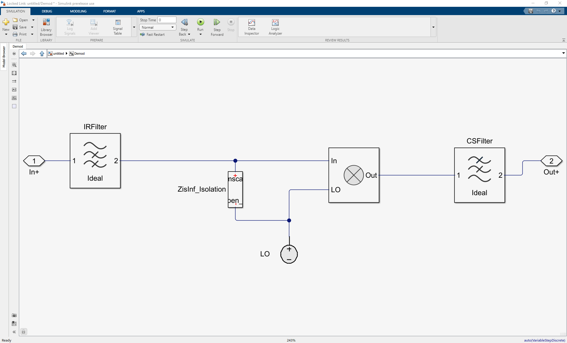
Look under the mask of the Demodulator block. This block consists of an ideal filter and a channel select filter and an LO for frequency up or down conversion. The stop time for the simulation is zero. To simulate time-varying results, you must change the stop time.

Export to RF Blockset Testbench

Use the Export button to export the receiver to an RF Blockset measurement testbench. Measuring properties such as gain, noise figure, and intercept points (IPs) in RF systems is crucial to the system design and analysis processes. Such measurements are accomplished by placing a DUT in a testbench. Use the testbenches blocks to measure the RF properties and verify the response of the DUT.

The RF Blockset testbench consists of two subsystems: RF Measurement Unit and Device Under Test.

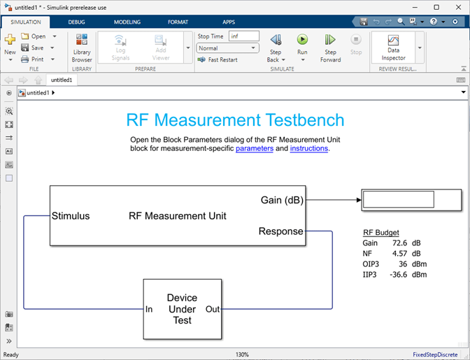
The Device Under Test subsystem contains the superheterodyne receiver you exported from the RF Budget Analyzer app. Double-click the Device Under Test subsystem to look inside.

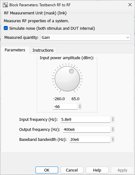
Double-click the RF Measurement Unit subsystem to see the system parameters. By default, the RF Blockset testbench verifies the gain.

Verify Gain, Noise Figure, and IP3 Using RF Blockset Testbench

You can verify the gain, noise figure, and IP3 measurements using the RF Blockset testbench.

By default, the model verifies the gain of the DUT. Run the model to check the gain. The simulated gain value matches the cascade transducer gain value from the app. The scope shows an output power of approximately 6.7 dB at 400 MHz that matches the output power value in the RF Budget Analyzer app.

The RF Blockset testbench calculates the spot noise figure. The calculation assumes a frequency-independent system within a given bandwidth. To simulate a frequency-independent system and calculate the correct noise figure value, you must reduce the broad bandwidth of 20 MHz to a narrow bandwidth.

To do so, first, stop all simulations. Double-click the RF Measurement Unit subsystem. This action opens the RF measurement unit parameters. In the Measured Quantity parameter drop-down list, select NF (noise figure). In the Parameters tab, set the Baseband bandwidth (Hz) parameter to 2000 Hz. Click Apply. To learn more about how to manipulate noise figure verification, click the Instructions tab.

Run the model again to check the noise figure value. The testbench noise figure value matches the cascade noise figure value from the RF Budget Analyzer app.

IP3 measurements rely on the creation and measurement of intermodulation tones that are usually small in amplitude and may be below the DUT's noise floor. For accurate IP3 measurements, clear the Simulate noise check box.

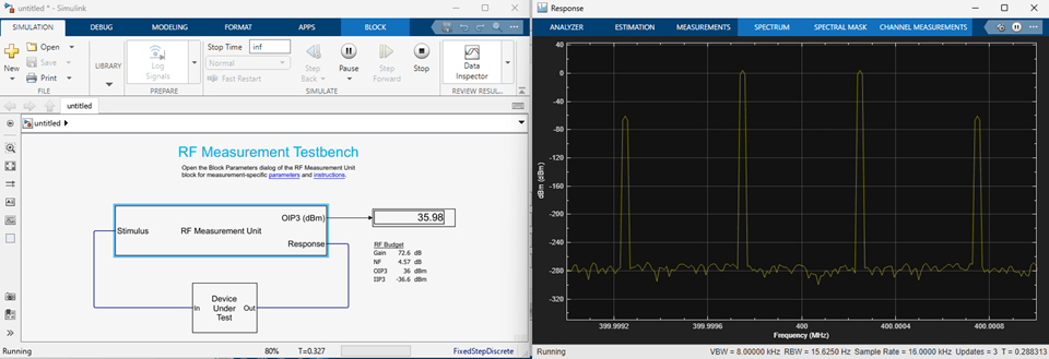
To verify OIP3, stop all simulations. Open the dialog box of the RF Measurement Unit block. Clear the Simulate noise (both stimulus and DUT internal) check box. Change the Measured Quantity parameter to IP3. Keep the IP Type as Output referred. To learn more about how to manipulate OIP3 verification, click the Instructions tab. Click Apply.

Run the model. The testbench OIP3 value matches the cascade OIP3 value from the app.

To verify IIP3, stop all simulations. Open dialog box of the RF Measurement Unit block. Clear the Simulate noise (both stimulus and DUT internal) check box. Change the Measured Quantity parameter to IP3. Change the IP Type to Input referred. To learn more about how to manipulate IIP3 verification, click the Instructions tab. Click Apply.

Run the model again to check the IIP3 value.

To sum up, in this example, you have seen how to build, analyze, and verify a superheterodyne receiver. Similarly, you can build and analyze an RF chain programmatically in the MATLAB command line or interactively using the RF Budget Analyzer app, and generate circuit envelope models for system-level simulation.

References

[1] Hongbao Zhou, Bin Luo. " Design and budget analysis of RF receiver of 5.8GHz ETC reader" Published at Communication Technology (ICCT), 2010 12th IEEE International Conference, Nanjing, China, November 2010.

[2] Bin Luo, Peng Li. "Budget Analysis of RF Transceiver Used in 5.8GHz RFID Reader Based on the ETC-DSRC National Specifications of China" Published at Wireless Communications, Networking and Mobile Computing, WiCom '09. 5th International Conference, Beijing, China, September 2009.