RF Budget Analyzer
Analyze gain, noise figure, IP2, and IP3 of cascaded RF elements and export to RF Blockset
Description
The RF Budget Analyzer app analyzes the gain, noise figure, and nonlinearity of proposed RF system architecture.
Using this app, you can:
Build a cascade of RF elements.
Calculate the per-stage and cascade output power, gain, noise figure, SNR, and IP3 of the system.
Compute nonlinear effects such as output power, IP2, NF, and SNR using harmonic balance analysis.
Compare Friis and harmonic balance budget results.
Plot:
rfbudget
results across bandwidths and over stages.S-parameters of the RF System on a Smith® Chart and a polar plot.
Magnitude, phase and real, and imaginary parts of S-parameters of the RF System and over stages.
Export:
Per-stage and cascade values to the MATLAB® workspace.
System design to RF Blockset™ for simulation.
System design to the RF Blockset Testbench as a device under test (DUT) subsystem and verify the results using simulation.
System design to
rfsystem
System object™.
Visualize:
Budget results, S-parameters over stages and frequencies.
Amplifier power characteristics. (since R2023a)
One- and two-tone harmonic balance results of the RF budget chain. (since R2023b)
Mixer spurs and spur-free zones of the IMT Mixer. (since R2024a)
Treat an N-port element with multiple ports as a 2-port element. (since R2024b)
Increase the number of harmonics for higher fidelity harmonic balance (HB) simulation and reduce the number of harmonics for faster harmonic balance simulation. (since R2024b)
Note
The RF Budget Analyzer app assumes a reference temperature of 290 K when calculating the SNR of an RF chain.
If you use:
A stripline element in your system, then the app does not support exporting your system to RF Blockset.
An antenna element, the app does not support exporting to a testbench in the RF Blockset using the Measurement Testbench option.
More
Available Blocks
The app toolstrip contains these nonlinear elements that you can use to create an RF system:
Amplifier
Modulator
Demodulator
Generic
Mixer IMT
The app toolstrip contains these linear elements that you can use to create an RF system:
S-Parameters
Filter
Transmission Line
Series RLC
Shunt RLC
Attenuator
Transmitter Antenna
Receiver Antenna
Transmit-Receive Antenna
LC Ladder
Phase Shift
Mutual Inductor
Available Templates
The app toolstrip contains these templates that you can use to design a transmitter or a receiver system:
Receiver
Transmitter
Open the RF Budget Analyzer App
MATLAB Toolstrip: On the Apps tab, under RF and Mixed-Signal, click the app icon.
MATLAB command prompt: Enter
rfBudgetAnalyzer
.
Examples
RF Transmitter System Analysis
Design and analyze an RF transmitter using the RF Budget Analyzer app.
Enter rfBudgetAnalyzer
to open the app.
Select New and then select select Transmitter to use the transmitter template to create a basic transmitter.
The transmitter template is displayed as follows.
In System Parameters, specify the RF transmitter requirements:
Input Frequency —
815
MHzAvailable Input Power —
0
dBmSignal Bandwidth —
100
MHz
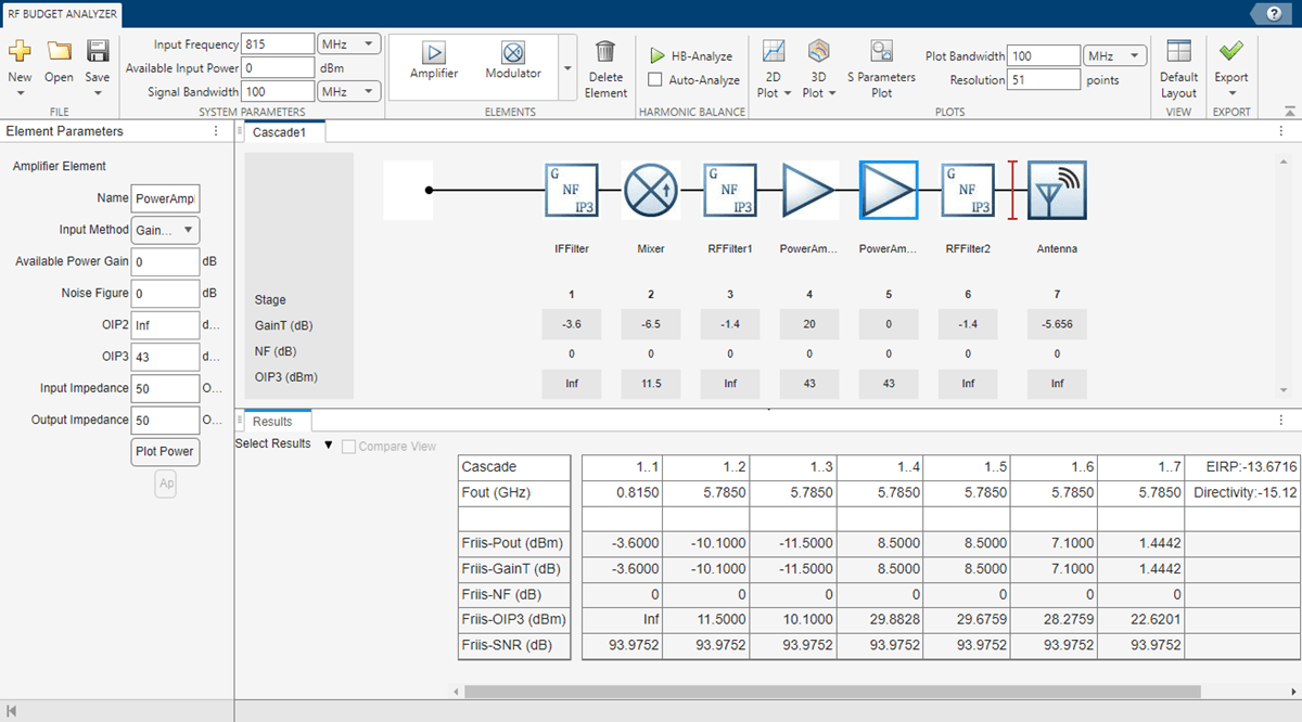
Click the IFAmplifier
in the design canvas and delete the element using the Delete Element button on the toolstrip.
Add a Generic element in the place of the IFAmplifier
using the toolstrip. In the Element Parameters pane, specify:
Name —
IFFilter
Available Power Gain — –
3.6
dBSelect Apply.
Click the Modulator element. In the Element Parameters pane, specify:
Name —
Mixer
Available Power Gain — –
6.5
dBOIP3 —
11.5
dBmLO Frequency —
4.97
GHzConverter Type —
Up
Select Apply.
Delete the S-Parameters element named BandpassFilter
. Add a Generic element. In the Element Parameters pane, specify:
Name —
RFFilter1
Available Power Gain — –
1.4
dBSelect Apply.
Select the PowerAmplifier
element and in the Element Parameters pane, specify:
Name —
PowerAmplifier1
Available Power Gain —
20
dBOIP3 —
43
dBmSelect Apply.
Add another Amplifier element using the toolstrip. In the Element Parameters pane, specify:
Name —
PowerAmplifier2
Available Power Gain —
20
dBOIP3 —
43
dBmSelect Apply.
Add another Generic element. In the Element Parameters pane, specify:
Name —
RFFilter2
Available Power Gain — –
1.4
dBSelect Apply.
Save the system. The app saves the system in a MAT file.
Plot the output power of the transmitter using the 3D Plot button. Select 3D Plot and choose Output Power - Pout
.
Select the PowerAmplifer1
element and from the Element Parameters pane, and then click the Plot Power Characteristics button to plot amplifier power characteristics of the PowerAmplifer1
element. Alternatively, to plot the amplifier power characteristics of the PowerAmplifer1
element, select the PowerAmplifer1
element and using the 2-D Plot button, choose Plot Power Characteristics
.(Since 2023a)
Use Transmit Antenna in RF Transmitter Design
This example uses an RF transmitter design from the RF Transmitter System Analysis example.
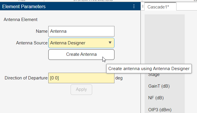
Follow the RF Transmitter System Analysis example to design an RF transmitter. Select the antenna element from the Elements section and add the element at end of this RF transmitter. In the Element Parameters pane, select Antenna Designer
from the Antenna Source drop-down list.
Click Create Antenna in the Element Parameters pane.
The Antenna Designer app opens. Click New to explore the antenna library. This example uses a dipoleFolded
antenna element with a center frequency of 815
MHz. To do this, select Folded
element from the Antenna Gallery, set Design Frequency to 815
MHz, and click Accept.
The updated antenna shows in the window.
Click Update Element to update the Antenna
element in the RF Budget Analyzer app. Click OK in the Confirm Update dialog box.
The Antenna Designer app window closes and the Antenna
element is updated in the RF Budget Analyzer app. The Results pane is automatically updated for Friis analysis with EIRP
and Directivity
of the Antenna
element.
RF Receiver System Analysis
Design and analyze an RF receiver using the RF Budget Analyzer app.
Enter rfBudgetAnalyzer
to open the app.
Click the New button and select Receiver to use the receiver template option to create a basic receiver.
The receiver template is displayed as follows:
In System Parameters, specify the RF receiver requirements:
Input Frequency —
5.745
MHzAvailable Input Power — –
65
dBmSignal Bandwidth —
100
MHz
Click RFFilter
in the design canvas. This RFFilter
is an S-parameters element. It accepts a Touchstone® file in the S2P file type. Update the Element parameters pane as follows:
Name:
BandpassFilter
S2P file: Choose an S2P file by clicking the Browse button.
Select Apply.
Click the RFAmplifier
element. In the Element Parameters pane, specify the element requirements:
Name —
LNA1
Available Power Gain —
12
dBOIP3 —
20
dBmSelect Apply.
Add another Amplifier element using the toolstrip. In the Element Parameters pane, specify the element requirements:
Name —
LNA2
Available Power Gain —
12
dBOIP3 —
20
dBmSelect Apply.
Add a Generic element. In the Element Parameters pane, specify the element requirements:
Name —
IRFilter
Available Power Gain — –
4.05
dBSelect Apply.
Click the Demodulator
element. In the Element Parameters pane, specify the element requirements:
Name —
Mixer
Available Power Gain — –
6.5
dBOIP3 —
11.5
dBmLO Frequency —
4.93
GHzConverter Type —
Down
Select Apply.
Delete the IFFilter
, S-parameters element. Add a Generic element in its place. In the Element Parameters pane, specify the element requirements:
Name —
CSFilter
Available Power Gain — –
9.55
dBSelect Apply.
Click the IFAmplifier
element. In the Element Parameters pane, specify the element requirements:
Name —
PowerAmp1
Available Power Gain —
16
dBOIP3 —
26
dBmSelect Apply.
Add two more Amplifier elements. For each element, in the Element Parameters panes specify the element requirements:
Name —
PowerAmp2
|PowerAmp3
Available Power Gain —
16
dB |20
dBOIP3 —
26
dBm |33
dBmSelect Apply.
Save the system. The app saves the system in a MAT file.
Plot the output OIP3 of the receiver using the 3D Plot button. Select the 3D Plot button and choose Output Third-Order Intercept Point - OIP3
.
Compare Friis and Harmonic Balance Solver
Create an amplifier with a gain of 4 dB.
a = amplifier('Gain',4);
Create a modulator with an OIP3 of 13 dBm.
m = modulator('OIP3',13);
Create an nport
using passive.s2p
.
n = nport('passive.s2p');
Create an RF element with a gain of 10 dB.
r = rfelement('Gain',10);
Calculate the rfbudget
of a series of RF elements at an input frequency of 2.1 GHz, an available input power of -30 dBm, and a bandwidth of 10 MHz.
b = rfbudget([a m r n],2.1e9,-30,10e6);
Run this command in the command window, to open the system in RF Budget Analyzer app.
show(b)
Set OIP2 value of Amplifier
to 60
dBm using Elements Parameters pane and select Apply. In System Parameters section, set the Available Input Power to 50
dBm and run harmonic balance analysis using HB-Analyze button.
The results are displayed as shown below.
Select Auto-Analyze checkbox from the Harmonic Balance section to automatically recompute the harmonic balance analysis calculations.
Set OIP2 value of RFelement
as 50
dBm using Elements Parameters pane and select Apply.
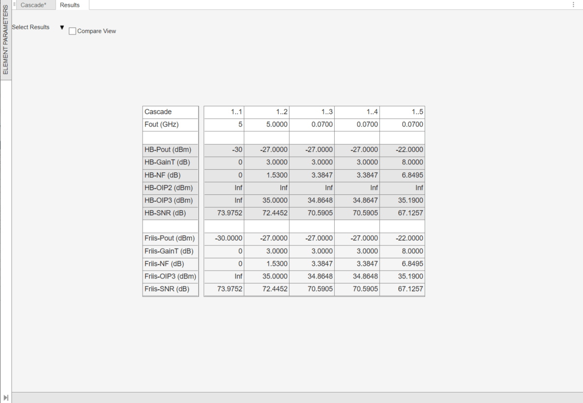
Select Compare View checkbox in the Results pane to compare the calculated Friis and harmonic balance solver results. You can use Select Results drop-down from the Results pane to filter the results and to compare between Friis and harmonic balance solver.
Design Input Matching Network Using Transmission Line Element
Design an input matching network for a two-stage amplifier using the Transmission Line element in the RF Budget Analyzer app.
Enter rfBudgetAnalyzer
to open the app.
In System Parameters, specify the requirements:
Input Frequency —
2.45
GHzAvailable Input Power —
0
dBmSignal Bandwidth —
2
GHz
Add two Transmission Line elements. In the Element Parameters pane, specify:
Name —
Microstrip1
|Microstrip2
Type —
Microstrip
| Microstrip
Width —
0.0034173
|0.0034173
metersHeight —
0.001524
|0.001524
metersThickness —
3.5e-06
|3.5e-06
metersEpsilonR —
3.48
|3.48
LossTangent —
0.0037
|0.0037
metersSigmaCond —
Inf
|Inf
S/mLineLength —
0.0089
|0.0147
metersStubMode —
Shunt
|NotAStub
Termination —
Open
Select Apply.
Add two S-Parameters elements. In the Element Parameters pane, specify:
Name —
Sparams1
|Sparams2
Load the Touchstone® file (f551432p.s2p
) to the S-Parameters elements provided in this example and select Apply.
Plot the input reflection coefficient of the system using the 3D Plot button. Select the 3D Plot button, choose S-Parameters
and select S11
.
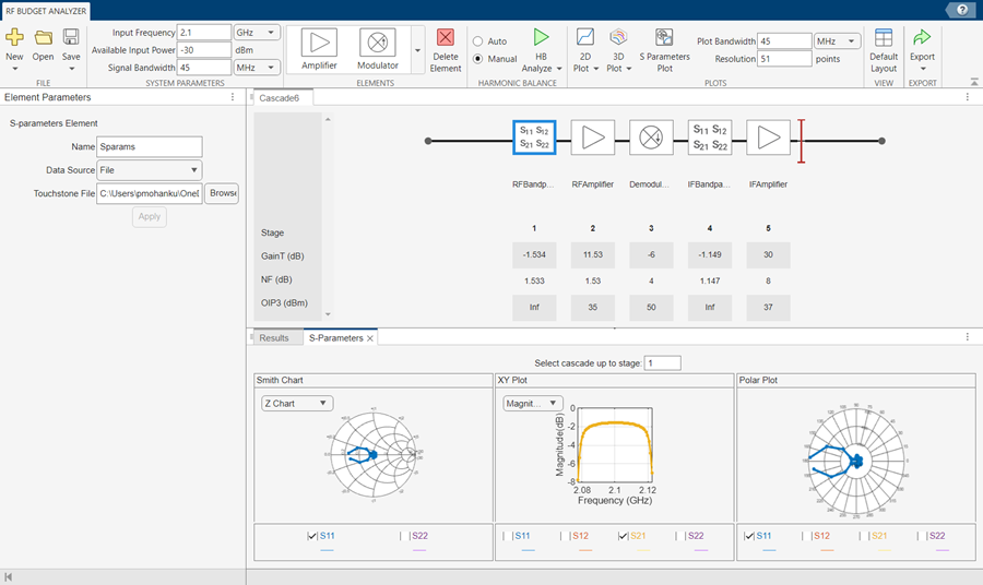
Plot S-Parameters, Output Power, and Transducer Gain of RF System
Design an RF system and plot S-parameters, output power, and transducer gain using RF Budget Analyzer app.
Enter rfBudgetAnalyzer
to open the app.
In System Parameters, specify the requirements:
Input Frequency —
2.1
GHzAvailable Input Power —
-30
dBmSignal Bandwidth —
45
MHz
Add a S-Parameters element. In the Element Parameters, specify:
Name —
RFBandpassFilter
Load the Touchstone® file (RFBudget_RF.s2p
) to the S-Parameters element provided in this example and select Apply.
Add an Amplifier element. In the Element Parameters, specify:
Name —
RFAmplifier
Available Power Gain —
11.53
dBNF —
1.53
dBOIP3 —
35
dBmSelect Apply.
Add the Demodulator element. In the Element Parameters, specify:
Name —
Demodulator
Available Power Gain —
-6
dBNF —
4
dBOIP3 —
50
dBmLO Frequency —
2.03
GHzConverter Type —
Down
Select Apply.
Add another S-Parameters element. In the Element Parameters, specify:
Name —
IFBandpassFilter
Load the Touchstone file (RFBudget_IF.s2p
) to the S-Parameters element provided in this example and select Apply.
Add another Amplifier element. In the Element Parameters, specify:
Name —
IFAmplifier
Available Power Gain —
30
dBNF —
8
dBOIP3 —
37
dBmSelect Apply.
Save the system. The app saves the system in a MAT file.
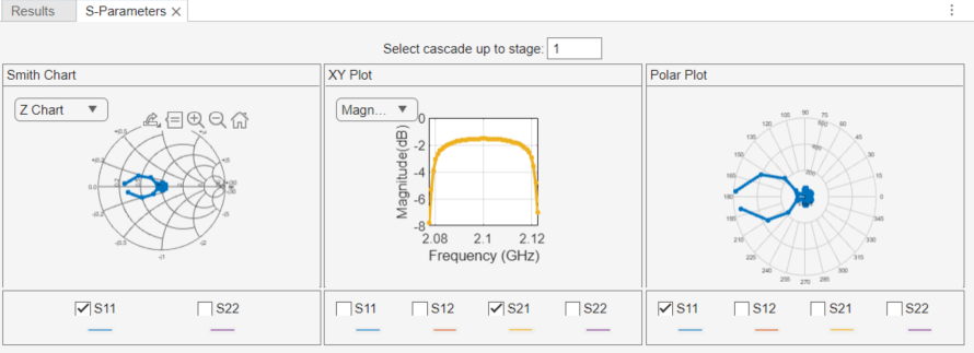
Select S-Parameters Plot button. This allows you to plot Smith® chart, polar plot, magnitude, phase and real, and imaginary parts of S-parameters of the RF System and over stages.
Set the Plot Bandwidth to 75
and Resolution to 250
under Plots section.
The S-parameters data is displayed as follows.
Select Phase (deg)
from the drop-down menu of XY Plot in S-Parameters pane to plot the phase of the S21.
The phase plot is displayed as shown.
Plot the output power of the RF system using the 2D Plot button. Select 2D Plot button and choose Output Power - Pout
. 2-D output power is displayed.
Plot the transducer gain of the RF system using the 2D Plot button. Select 2D Plot button and choose Transducer Gain - GainT
.
Perform HB Analysis on RF Receiver Designed Using rfsystem
Design an RF receiver using the rfsystem
system object. View the object in the the RF Budget Analyzer app to perform harmonic balance (HB) analysis.
Create fifth- and seventh-order bandpass RF filters.
f1 = rffilter('ResponseType','Bandpass','FilterOrder',5, ... 'PassbandFrequency',[4.85 5.15]*1e9); f2 = rffilter('ResponseType','Bandpass','FilterOrder',7, ... 'PassbandFrequency',[10 130]*1e6);
Create two amplifier objects with 3
dB and 5
dB gain, respectively.
a1 = amplifier('Gain',3,'NF',1.53,'OIP3',35); a2 = amplifier('Gain',5,'NF',8,'OIP3',37);
Create a modulator with a local frequency of 4.93
GHz.
d = modulator('Gain',0,'NF',4,'OIP3',50,'LO',4.93e9, ... 'ConverterType','Down');
Design an RF receiver with the budget elements at an input frequency of 5
GHz, an available input power of – 30
dBm, and a bandwidth of 10
MHz.
rfb = rfbudget([f1 a1 d f2 a2],5e9,-30,10e6);
Create an RF system for the RF receiver using the rfbudget
object.
rfs = rfsystem(rfb);
Open an RF Blockset model of the designed RF system using the open_system
function.
open_system(rfs)
Type rfBudgetAnalyzer(rfs) command at the MATLAB® command line to open this RF system in the RF Budget Analyzer app.
To conduct HB analysis in the app, click the HB-Analyze button.
Related Examples
Programmatic Use
rfBudgetAnalyzer
rfBudgetAnalyzer
opens the RF Budget Analyzer app
to analyze the stage-wise and total gain, noise figure, and nonlinearity (IP3) of an
RF system.
rfBudgetAnalyzer(rfbmat)
opens an RF system saved using the
RF Budget Analyzer app. rfbmat
is a MAT
file.
rfBudgetAnalyzer(rfb)
opens an RF system saved using the
rfbudget
object rfb
in the RF Budget Analyzer app.
rfBudgetAnalyzer(rfs)
opens an RF system saved using the
rfsystem
system object rfs
in the RF Budget Analyzer
app.
Tips
The RF Budget Analyzer app accepts
0
Hz as Input Frequency for a system. You can set the Input Frequency in the System Parameters section.The RF Budget Analyzer app does not accept
0
Hz as LO Frequency. This is applicable to Modulator and Demodulator elements.The output frequencies from the RF Budget Analyzer app are always positive.
The Filter element allows you to use only the
'Transfer function'
implementation when you set the Filter Type to'InverseChebyshev'
in the Element Parameters pane.To design an antenna element using the RF Budget Analyzer app, in the Antenna Element pane, set Antenna Source to
Isotropic radiator
.You can also design an antenna element using the Antenna Designer app or an antenna object. To use the Antenna Designer app or the antenna object, you need Antenna Toolbox™ license.Antenna elements designed using a default antenna object require larger memory. To speed up the simulation, design your antenna element at a high frequency,
2
GHz or more.
References
[1] Pozar, David M. Microwave Engineering. 4th ed. Hoboken, NJ: Wiley, 2012.
Version History
Introduced in R2016aR2024b: Treat N-port element with multiple ports as 2-port element
You can now use the RF Budget Analyzer app to treat an N-port element with multiple ports as a 2-port element.
R2024b: Limit number of harmonics in harmonic balance (HB) simulation
You can now use the RF Budget Analyzer app to increase the number of harmonics for higher fidelity HB simulation and reduce the number of harmonics for faster HB simulation.
R2024a: Specify AM/AM-AM/PM amplifier data in RF Budget Analyzer app
You can now use the RF Budget Analyzer app to specify AM/AM-AM/PM amplifier data.
To specify AM/AM-AM/PM amplifier data, first select
Amplifier from the Elements tab
and set Input Method to AM/AM-AM/PM
Table
. This enables AM/AM-AM/PM Table
parameter. Input your AM/AM-AM/PM data to AM/AM-AM/PM Table
parameter.
R2024a: Visualize spur and spur-free zones in IMT mixer using rfplot
and RF Budget Analyzer app
You can now use the RF Budget Analyzer app to visualize the spur and
spur-free zones in a mixerIMT
object.
R2023b: Visualize one- and two-tone harmonic balance results of RF budget chain
The rfplot
function and the RF Budget Analyzer app now support visualizing one- and
two-tone harmonic balance results of the RF budget chain.
R2023b: Recommended over analyze
R2023a: Mutual inductor, lumped transmission line, and amplifier power characteristics
The RF Budget Analyzer app now supports:
Visualizing the amplifier power characteristics of an
amplifier
element.Adding
mutualInductor
andtxlineLumped
elements to the RF chain.
R2022b: Model stripline element and use network parameter object to model S-parameter
Use the RF Budget Analyzer app to:
Model a stripline element to your RF system by selecting Transmission line from the Elements tab and setting Type to
Stripline
.Model an S-parameters element with a network parameter object created at the MATLAB command line. To design the S-parameter element, first select S-parameters from the Elements tab, and then set Data Source to
Object
.
R2022a: Model IMT mixer and transmit-receive elements and model amplifier element using network parameter object
Use the RF Budget Analyzer app to:
Model a IMT mixer by selecting Mixer IMT element from the element pane.
Model an antenna in transmit-receive configuration by selecting TxRxAntenna element from the element pane.
Model an amplifier element with a network parameter object created at the MATLAB command line. To design an amplifier element, first select Amplifier from the Elements tab and set Input Method to
Network Parameters
. Then, set Data Source toObject
.
R2022a: Export RF system to rfsystem
object
Use the RF Budget Analyzer app to export your RF system to
rfsystem
object. To export, select Export,
and click Export to rfsystem.
MATLAB Command
You clicked a link that corresponds to this MATLAB command:
Run the command by entering it in the MATLAB Command Window. Web browsers do not support MATLAB commands.
Select a Web Site
Choose a web site to get translated content where available and see local events and offers. Based on your location, we recommend that you select: .
You can also select a web site from the following list
How to Get Best Site Performance
Select the China site (in Chinese or English) for best site performance. Other MathWorks country sites are not optimized for visits from your location.
Americas
- América Latina (Español)
- Canada (English)
- United States (English)
Europe
- Belgium (English)
- Denmark (English)
- Deutschland (Deutsch)
- España (Español)
- Finland (English)
- France (Français)
- Ireland (English)
- Italia (Italiano)
- Luxembourg (English)
- Netherlands (English)
- Norway (English)
- Österreich (Deutsch)
- Portugal (English)
- Sweden (English)
- Switzerland
- United Kingdom (English)
Asia Pacific
- Australia (English)
- India (English)
- New Zealand (English)
- 中国
- 日本Japanese (日本語)
- 한국Korean (한국어)