amplifier

Create two-port amplifier element

Description

Use the amplifier object to create a two-port amplifier element or to analyze a commercial off-the-shelf (COTS) amplifier. You can also use the amplifier object to model an amplifier in an RF system created using an rfbudget object or the RF Budget Analyzer app and, then export this element to RF Blockset™ or to rfsystem System object™ for circuit envelope analysis.

Creation

Syntax

amp = amplifier

amp = amplifier(Name=Value)

Description

amp = amplifier creates an amplifier object with default property values.

example

amp = amplifier(Name=Value) sets amplifier object properties using one or more name-value arguments. You can specify multiple name-value arguments.

example

Properties

expand all

`Name` — Name of amplifier
`'Amplifier'` (default) | character vector | string scalar

Name of amplifier, specified as a character vector. All names must be valid MATLAB^® variable names.

Example: Name='amp'

`Model` — Amplifier model
`'cubic'` (default) | `'sparam'` | `'ampm'`

Since R2024b

Amplifier model, specified as one of the following:

'cubic' — Cubic polynomial model. When you set this value, the amplifier object uses the Gain, Zin, Zout, and NF properties to compute gain, matching, and noise.
'sparam' — S-parameter model. When you set this value, the amplifier object uses the NetworkData and NoiseData properties to compute gain, matching, and noise. Input the S-parameter data using the NetworkData or FileName property.
'ampm' — AM/PM-AM/PM model. When you set this value, the amplifier object uses AM/AM–AM/PM data to characterize the amplifier. Input AM/AM–AM/PM data using the AMPMTable property.

Example: Model='ampm'

`Gain` — Available power gain
`0` (default) | real finite scalar

Available power gain, specified as a real finite scalar in dB.

Example: Gain=10

`NF` — Noise figure
`0` (default) | real finite nonnegative scalar

Noise figure, specified as a real finite nonnegative scalar dB.

Example: NF=-10

`OIP2` — Second-order output-referred intercept point
`Inf` (default) | real scalar

Second-order output-referred intercept point, specified as a real scalar in dBm.

Example: OIP2=8

`OIP3` — Third-order output-referred intercept point
`Inf` (default) | real scalar

Third-order output-referred intercept point, specified as a real scalar in dBm.

Example: OIP3=10

`Zin` — Input impedance
`50` (default) | positive real part finite scalar

Input impedance, specified as a positive real part finite scalar in ohms. You can also use a complex value with a positive real part.

Example: Zin=40

`Zout` — Output impedance
`50` (default) | positive real part finite scalar

Output impedance, specified as a scalar in ohms. You can also use a complex value with a positive real part.

Example: Zout=40

`FileName` — Name of two-port Touchstone file
`''` (default) | string scalar | character vector

Name of the two-port Touchstone file from which to extract the NetworkData and the NoiseData properties, specified as a string scalar or character vector.

Example: FileName='default.s2p'

`NetworkData` — Network Data
network parameter object

Network data of the amplifier, specified as a two-port network parameter object. The network parameter objects are of the type:

Network parameter object defines the frequency-dependent gain and impedance matching for the amplifier, typically, a sparameters object from a two-port Touchstone file. To specify a frequency-independent network data, set the NetworkData property to []. This resets network data to a frequency-independent two-port network object defined by the Gain, Zin, and Zout properties.

Example: NetworkData=nd

`NoiseData` — Noise Data
`noiseParameter` object

Noise data of the amplifier, specified as a noiseParameters object. The noiseParameter object contains a frequency-dependent noise figure loaded from a two-port Touchstone file or built at the MATLAB® command line. To specify a frequency-independent noise figure, set the NoiseData to [].

Example: NoiseData=np

`AMPMTable` — Lookup table entries
`[ -25, 5, -1; -10, 20, -2; 0, 27, 5; 5, 28, 12 ]` (default) | real M-by-3 matrix

Since R2023b

Lookup table entries, specified as a real M-by-3 matrix. M must be a positive scalar. The first column of the matrix represents the input power, and the values in this column must increase monotonically. The second column of the matrix represents the output power in dBm in the AM/AM-AM/PM model and the third column represents the phase change in degrees in the model. The values in the second and third columns are related to the absolute value of the power of the input signal represented in the first column.

To enable the AMPMTable property, set Model to ampm.

Example: AMPMTable=[ -25, 5, 0; -10, 20, -2; 0, 27, 5; 5, 28, 12 ]

`NumPorts` — Number of ports
`2` (default) | scalar integer

This property is read-only.

Number of ports, returned as a scalar integer.

`Terminals` — Names of port terminals
`{'p1+' 'p2+' 'p1-' 'p2-'}` (default) | cell vector

This property is read-only.

Names of port terminals, returned as a cell vector.

Object Functions

`clone`	Create copy of existing circuit element or circuit object
`rfplot`	Plot cumulative RF budget result vs. cascade input frequency and amplifier power characteristics

Examples

collapse all

Analyze COTS Amplifier

Open Live Script

Use the RF Toolbox amplifier object to model a Qorvo CMD240 COTS amplifier. First, use the sparameter object to capture the S-parameter data from the CMD240 data file (Copyright (c) Qorvo, Inc., reproduced with permission).

S = sparameters('cmd240-sparameters.s2p');
rfplot(S)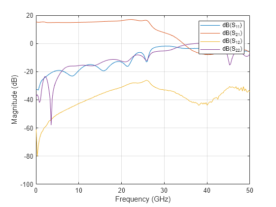

$Figure contains an axes object. The axes object with xlabel Frequency (GHz), ylabel Magnitude (dB) contains 4 objects of type line. These objects represent dB(S_{11}), dB(S_{21}), dB(S_{12}), dB(S_{22}).$

Then use the noiseParameters object to build the noise data.

NF = [4 2.9 2.2 1.8 2.2 2 2.1 2.3 2.4 3.1 3.7];
freqs = (2:2:22)*1e9;
nd = noiseParameters(NF,freqs,50)

nd = 
  noiseParameters with properties:

    Frequencies: [11x1 double]
           Fmin: [11x1 double]
       GammaOpt: [11x1 double]
             Rn: [11x1 double]

Create an amplifier using the CMD240 data file and add the noise data to the amplifier.

a1 = amplifier('FileName','cmd240-sparameters.s2p','OIP3',27.8);
a1.NoiseData = nd % clears FileName since there is no noise in the file.

a1 = 
  amplifier: Amplifier element

           Name: 'Amplifier'
          Model: 'sparam'
       FileName: ''
    NetworkData: [1x1 sparameters]
      NoiseData: [1x1 noiseParameters]
           OIP2: Inf
           OIP3: 27.8000

Alternatively, you can use the nport object to hold both the S-parameter and the noise data and then use the rfwrite function to create a Touchstone file.

n = nport(NetworkData=S,NoiseData=nd);
rfwrite(n,'CMD240withNF.s2p','Format','RI')
a = amplifier('FileName','CMD240withNF.s2p','OIP3',27.8);

Use the rfbudget object to compare harmonic balance analysis with Friis analysis.

b = rfbudget(a,10e9,-30,1e3,'Solver','HarmonicBalance');
b.Friis

ans = struct with fields:
       OutputPower: -15.0349
    TransducerGain: 14.9651
                NF: 2.2000
              IIP2: []
              OIP2: []
              IIP3: 12.7828
              OIP3: 27.8000
               SNR: 111.7752

b.HarmonicBalance

ans = struct with fields:
         OutputPower: -15.0353
      TransducerGain: 14.9647
                  NF: 2.1995
                IIP2: Inf
                OIP2: Inf
                IIP3: 12.7825
                OIP3: 27.7990
                 SNR: 111.7756
    OneToneSolutions: {[1x1 rf.internal.rfengine.analyses.solution]}
    TwoToneSolutions: {[1x1 rf.internal.rfengine.analyses.solution]}

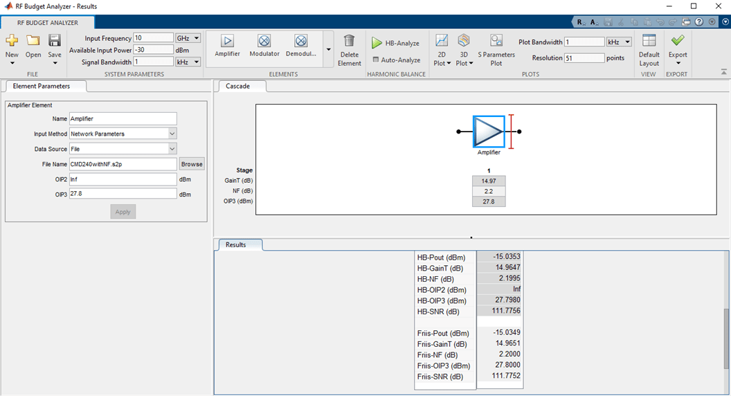
Gain is about 15 dB and noise figure is about 2.2 dB. This matches the product data sheet. For more information, see CMD240 product data sheet. You can verify this in RF Budget Analyzer app.

show(b)

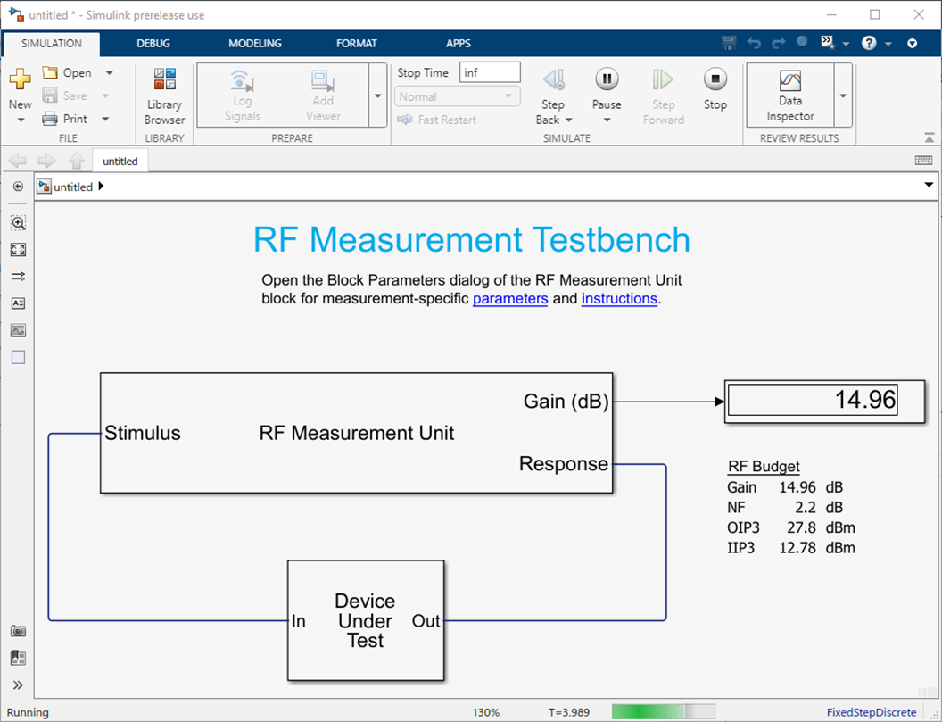
You can also use the exportTestbench function to verify with RF Blockset simulation. Type exportTestbench(b) command at the command line to open measurement testbench from RF budget object.

exportTestbench(b)

Click Run to see the Gain is about 15 dB.

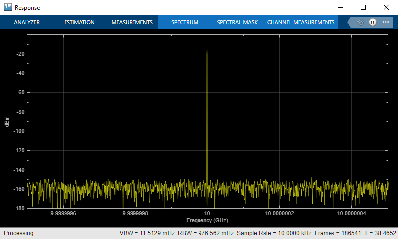
Set the Measured quantity of the RF Measurement Unit to NF and then click Run to see the noise figure is about 2.2 dB.

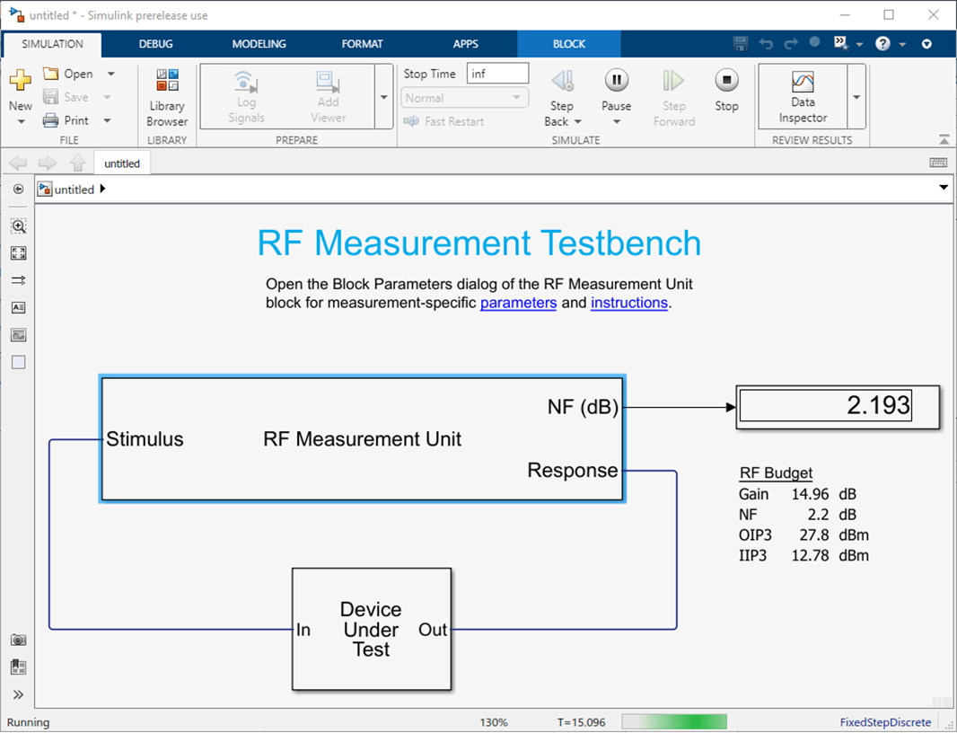
The amplifier response is displayed in the Spectrum Analyzer window.

Plot Amplifier Characteristics

Since R2023a

Open Live Script

Create an amplifier object.

amp = amplifier;

Plot the amplifier power characteristics at 2.1 GHz.

rfplot(amp,2.1e9)

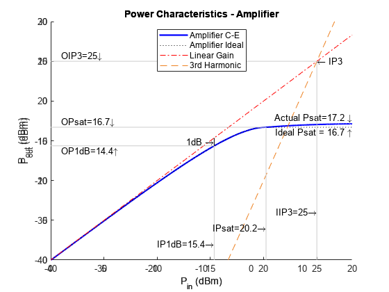
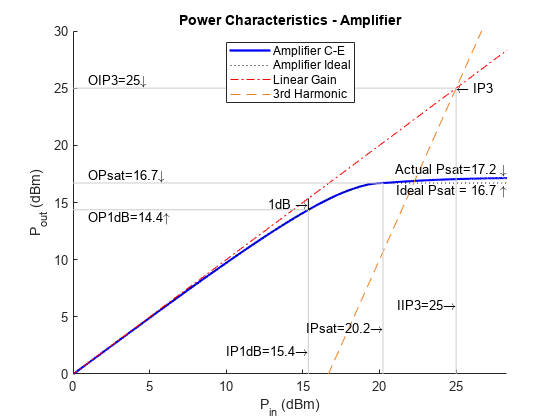
Set OIP3 of amplifier to 25 dBm.

amp.OIP3 = 25;

Plot the amplifier power characteristics at 2.1 GHz with nonlinearity.

rfplot(amp,2.1e9)

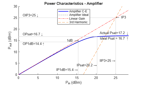
Plot the amplifier power characteristics on the axes specified in ax instead of the current axes.

f = figure;
ax = axes(f);
rfplot(ax,amp,2.1e9)

Figure contains an axes object. The axes object with title Power Characteristics - Amplifier, xlabel P_i_n (dBm), ylabel P_o_u_t (dBm) contains 21 objects of type line, text. These objects represent Amplifier C-E, Amplifier Ideal, Linear Gain, 3rd Harmonic.

Create Amplifier Element from Touchstone File Containing Noise Data

Open Live Script

Create an amplifier from the default.s2p Touchstone file.

a = amplifier(FileName='default.s2p')

a = 
  amplifier: Amplifier element

           Name: 'Amplifier'
          Model: 'sparam'
       FileName: 'default.s2p'
    NetworkData: [1x1 sparameters]
      NoiseData: [1x1 noiseParameters]
           OIP2: Inf
           OIP3: Inf

Define a measured noise figure, noise frequencies, and the reference impedance data.

NF = [4 3 2 2 2 2 2 2.5 2.5 3 3.5];
freqs = (2:2:22)*1e9;
z0 = 50;

Build the noise parameters from the measured NF data.

np = noiseParameters(NF,freqs,z0);

Add this noise data to the amplifier object.

a = amplifier(FileName='default.s2p',NoiseData=np)

a = 
  amplifier: Amplifier element

           Name: 'Amplifier'
          Model: 'sparam'
       FileName: ''
    NetworkData: [1x1 sparameters]
      NoiseData: [1x1 noiseParameters]
           OIP2: Inf
           OIP3: Inf

Create Amplifier Element

Open Live Script

Create an amplifier object named 'LNA' and has a gain of 10 dB.

a = amplifier(Name='LNA',Gain=10)

a = 
  amplifier: Amplifier element

     Name: 'LNA'
    Model: 'cubic'
     Gain: 10
       NF: 0
     OIP2: Inf
     OIP3: Inf
      Zin: 50
     Zout: 50

Amplifier Circuit

Open Live Script

Create an amplifier object with a gain of 4 dB. Create another amplifier object that has an output third-order intercept (OIP3) 13 dBm.

amp1 = amplifier('Gain',4);
amp2 = amplifier('OIP3',13);

Build a 2-port circuit using the amplifiers.

c = circuit([amp1 amp2])

c = 
  circuit: Circuit element

    ElementNames: {'Amplifier'  'Amplifier_1'}
        Elements: [1x2 amplifier]
           Nodes: [0 1 2 3]
            Name: 'unnamed'

RF Budget Analysis of Series of RF Elements

Open Live Script

Create an amplifier with a gain of 4 dB.

a = amplifier(Gain=4);

Create a modulator with an OIP3 of 13 dBm.

m = modulator(OIP3=13);

Create an N-port element using passive.s2p.

n = nport('passive.s2p');

Create an RF element with a gain of 10 dB.

r = rfelement(Gain=10);

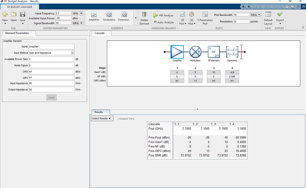
Calculate the RF budget of a series of RF elements at an input frequency of 2.1 GHz, an available input power of –30 dBm, and a bandwidth of 10 MHz.

b = rfbudget([a m r n],2.1e9,-30,10e6)

b = 
  rfbudget with properties:

               Elements: [1x4 rf.internal.rfbudget.Element]
         InputFrequency: 2.1 GHz
    AvailableInputPower: -30 dBm
        SignalBandwidth:  10 MHz
                 Solver: Friis      
             AutoUpdate: true

   Analysis Results
        OutputFrequency: (GHz) [  2.1    3.1    3.1     3.1]
            OutputPower: (dBm) [  -26    -26    -16   -20.6]
         TransducerGain: (dB)  [    4      4     14     9.4]
                     NF: (dB)  [    0      0      0  0.1392]
                   IIP2: (dBm) []                           
                   OIP2: (dBm) []                           
                   IIP3: (dBm) [  Inf      9      9       9]
                   OIP3: (dBm) [  Inf     13     23    18.4]
                    SNR: (dB)  [73.98  73.98  73.98   73.84]

Type the show command at the command window to display the analysis in the RF Budget Analyzer app.

show(b)

Version History

Introduced in R2017a

expand all

R2024b: Design amplifier using cubic polynomial model, AM/AM-AM/PM data, or S-parameter data

Use the new Model property in the amplifier object to design an amplifier using the cubic polynomial model, AM/AM-AM/PM data, or S-parameter data.

R2024b: `UseNetworkData` and `UseAMPMData` properties will be removed in future release

The UseNetworkData and UseAMPMData properties of the amplifier object will be removed in a future release. Use the new Model property instead.

When executing code with the amplifier object that uses the UseNetworkData and UseAMPMData properties, the software will replace these properties with the new Model property. The software assigns the Model property an sparam value if the original property is UseNetworkData and anampm value if the original property is UseAMPMData.

R2023b: Characterize amplifiers using AM/AM-AM/PM data

Use the UseAMPMData and AMPMTable properties to characterize an amplifier element using the AM/AM-AM/PM data. You can analyze this amplifier element using Friis or harmonic balance solvers with the rfbudget object.

R2023b: Recommended over `rfckt.amplifier`, `rfdata.ip3rfdata.power`, and `rfdata.nf`

amplifier is recommended over rfckt.amplifer, rfdata.ip3, rfdata.powerand rfdata.nf because it enables you to:

Create a two-port amplifier element.
Analyze a commercial off-the-shelf (COTS) amplifier.
Specify third-order intercept points and noise figure.
Characterize amplifiers using AM/AM-AM/PM data.
Build a circuit object with an amplifier element.
Model an amplifier in an RF chain created using an rfbudget object or the RF Budget Analyzer app, and then export this element to RF Blockset or to rfsystem System object for circuit envelope analysis.

R2022a: Model RF amplifier using network parameters from two-port Touchstone file

To model an RF amplifier element using network parameters from a two-port Touchstone file, specify the name of the file in the FileName property. The object extracts the values of the NetworkData and the NoiseData properties from this file.

amplifier

Description

Creation

Syntax

Description

Properties

Name — Name of amplifier 'Amplifier' (default) | character vector | string scalar

Model — Amplifier model 'cubic' (default) | 'sparam' | 'ampm'

Gain — Available power gain 0 (default) | real finite scalar

NF — Noise figure 0 (default) | real finite nonnegative scalar

OIP2 — Second-order output-referred intercept point Inf (default) | real scalar

OIP3 — Third-order output-referred intercept point Inf (default) | real scalar

Zin — Input impedance 50 (default) | positive real part finite scalar

Zout — Output impedance 50 (default) | positive real part finite scalar

FileName — Name of two-port Touchstone file '' (default) | string scalar | character vector

NetworkData — Network Data network parameter object

NoiseData — Noise Data noiseParameter object

AMPMTable — Lookup table entries [ -25, 5, -1; -10, 20, -2; 0, 27, 5; 5, 28, 12 ] (default) | real M-by-3 matrix

NumPorts — Number of ports 2 (default) | scalar integer

Terminals — Names of port terminals {'p1+' 'p2+' 'p1-' 'p2-'} (default) | cell vector

Object Functions

Examples

Analyze COTS Amplifier

Plot Amplifier Characteristics

Create Amplifier Element from Touchstone File Containing Noise Data

Create Amplifier Element

Amplifier Circuit

RF Budget Analysis of Series of RF Elements

Version History

R2024b: Design amplifier using cubic polynomial model, AM/AM-AM/PM data, or S-parameter data

R2024b: UseNetworkData and UseAMPMData properties will be removed in future release

R2023b: Characterize amplifiers using AM/AM-AM/PM data

R2023b: Recommended over rfckt.amplifier, rfdata.ip3rfdata.power, and rfdata.nf

R2022a: Model RF amplifier using network parameters from two-port Touchstone file

See Also

WeChat

`Name` — Name of amplifier
`'Amplifier'` (default) | character vector | string scalar

`Model` — Amplifier model
`'cubic'` (default) | `'sparam'` | `'ampm'`

`Gain` — Available power gain
`0` (default) | real finite scalar

`NF` — Noise figure
`0` (default) | real finite nonnegative scalar

`OIP2` — Second-order output-referred intercept point
`Inf` (default) | real scalar

`OIP3` — Third-order output-referred intercept point
`Inf` (default) | real scalar

`Zin` — Input impedance
`50` (default) | positive real part finite scalar

`Zout` — Output impedance
`50` (default) | positive real part finite scalar

`FileName` — Name of two-port Touchstone file
`''` (default) | string scalar | character vector

`NetworkData` — Network Data
network parameter object

`NoiseData` — Noise Data
`noiseParameter` object

`AMPMTable` — Lookup table entries
`[ -25, 5, -1; -10, 20, -2; 0, 27, 5; 5, 28, 12 ]` (default) | real M-by-3 matrix

`NumPorts` — Number of ports
`2` (default) | scalar integer

`Terminals` — Names of port terminals
`{'p1+' 'p2+' 'p1-' 'p2-'}` (default) | cell vector

R2024b: `UseNetworkData` and `UseAMPMData` properties will be removed in future release

R2023b: Recommended over `rfckt.amplifier`, `rfdata.ip3rfdata.power`, and `rfdata.nf`