Design Two-Stage Low Noise Amplifier Using Microstrip Transmission Line Matching Network

Open Live Script

This example shows how to use the RF Toolbox™ microstrip transmission line element to design two-stage low noise amplifier (LNA) for wireless local area network (WLAN) with an input and the output matching network (MNW) to maximize the power delivered through a 50-ohm load and the system.

Designing an input and output MNW is an important part of the amplifier design. The amplifier in this example has high gain and low noise. To minimize parasitic effect, this example uses the microstrip transmission line MNW with a single stub.

Define Microstrip Transmission Line Parameters

The microstrip transmission line parameters are chosen as follows.

Physical Height of conductor or dielectric thickness — 1.524 mm
Relative permittivity of dielectric — 3.48
Loss angle tangent of dielectric — 0.0037
Physical thickness of microstrip transmission line — 3.5 um

Design Input Matching Network Using Microstrip Transmission Line

The input matching network consists of one shunt stub and one series microstrip transmission line.

Create an input shunt stub microstrip transmission line with the physical length of 8.9 mm.

TL1 = txlineMicrostrip('Width',3.41730e-3,'Height',1.524e-3,'EpsilonR',3.48,'LossTangent',0.0037,...
    'LineLength',8.9e-3,'Thickness',0.0035e-3,'StubMode','Shunt','Termination','Open');

Create an input series microstrip transmission line with the physical length of 14.7 mm.

TL2 = txlineMicrostrip('Width',3.41730e-3,'Height',1.524e-3,'EpsilonR',3.48, 'LossTangent',0.0037,...
    'LineLength',14.7e-3,'Thickness',0.0035e-3);

Create and Extract Amplifier Object

Create and extract an amplifier object from the frequency dependent S-parameter data available in the specified file.

amp1 = nport('f551432p.s2p');

Define the frequency range.

freq = 2e9:10e6:3e9;

Create a two-stage amplifier and plot its S-parameter.

casamp = circuit([amp1,clone(amp1)],'amplifiers'); % amplifier ciruit without MNW.

Plot the S-Parameter over the frequency range from 2 – 3 GHz.

S2 = sparameters(casamp,freq);

Design Output Matching Network Using Microstrip Transmission Line

The output matching network consists of one shunt stub and one series microstrip transmission line.

Create an output series microstrip transmission line with the physical length of 22.47 mm.

TL3 = txlineMicrostrip('Width',3.41730e-3,'Height',1.524e-3,'EpsilonR',3.48, 'LossTangent',0.0037,...
    'LineLength',22.47e-3,'Thickness',0.0035e-3);

Create an output shunt stub microstrip transmission line with the physical length of 5.66 mm.

TL4 = txlineMicrostrip('Width',3.41730e-3, 'Height',1.524e-3,'EpsilonR',3.48, 'LossTangent',0.0037,...
    'LineLength',5.66e-3,'Thickness',0.0035e-3,'StubMode','Shunt','Termination','Open');

Plot Input Reflection Coefficients of Two-Stage LNA

To verify the simultaneous conjugate match at the input of the amplifier, plot the input reflection coefficients in dB for the amplifier circuit with and without a matching network.

Cascade the circuit elements by adding the input and the output MNW to the two-stage amplifier.

c = circuit([TL1, TL2,clone(amp1),clone(amp1),TL3, TL4]); % two-stage LNA with MNW

Plot the S-parameters and analyze the amplifier with and without the matching networks over the frequency range of 2.4 – 2.5 GHz.

figure
S3 = sparameters(c,freq); 
rfplot(S2,1,1)
hold on;
rfplot(S3,1,1)
legend('|S11| of Two-Stage LNA Without MNW','|S11| of Two-Stage LNA with MNW');
title('Input Reflection Coefficients of Two-Stage LNA');
grid on;

Figure contains an axes object. The axes object with title Input Reflection Coefficients of Two-Stage LNA, xlabel Frequency (GHz), ylabel Magnitude (dB) contains 2 objects of type line. These objects represent |S11| of Two-Stage LNA Without MNW, |S11| of Two-Stage LNA with MNW.

The calculated input return loss for the two-stage LNA with the input MNW is around 13 dB.

Plot Output Reflection Coefficients of Two-Stage LNA

To verify the simultaneous conjugate match at the output of the amplifier, plot output reflection coefficients in dB for both the two-stage LNA with and without a MNW.

figure
rfplot(S2,2,2)
hold on;
rfplot(S3,2,2)
legend('|S22| of Without MNW','|S22| of With MNW');
title('Output Reflection Coefficients of Two-Stage LNA');
grid on;

Figure contains an axes object. The axes object with title Output Reflection Coefficients of Two-Stage LNA, xlabel Frequency (GHz), ylabel Magnitude (dB) contains 2 objects of type line. These objects represent |S22| of Without MNW, |S22| of With MNW.

The calculated output return loss for the two-stage LNA with the output MNW is aroung 11 dB.

Plot Gain and Input Reflection Coefficients of Cascaded LNA

To verify the simultaneous conjugate match at the input and output of the amplifier, plot the input reflection coefficient and the gain parameters in dB for the two-stage LNA with the MNW.

figure;
rfplot(S3,1,1)
hold on;
rfplot(S3,2,1)
title('Gain and Input Reflection Coefficients of Cascaded LNA');
grid on;

$Figure contains an axes object. The axes object with title Gain and Input Reflection Coefficients of Cascaded LNA, xlabel Frequency (GHz), ylabel Magnitude (dB) contains 2 objects of type line. These objects represent dB(S_{11}), dB(S_{21}).$

The calculated amplifier gain, S21 is 34.5 dB, and the input reflection coefficient, S11 is around 13 dB.

Calculate and Plot Complex Load and Source Reflection Coefficients

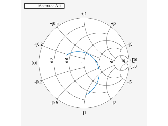
Calculate and plot all the complex load and source reflection coefficients for simultaneous conjugate match at all measured frequency data points that are unconditionally stable. These reflection coefficients are measured at the amplifier interfaces.

figure
smithplot(S3,1,1,'LegendLabels','Measured S11')

Figure contains an axes object. The hidden axes object contains an object of type line. This object represents Measured S11.

Calculate Ampifier Noise Figure

Use an rfbudget object to calculate the amplifier noise figure.

b = rfbudget( ...
    'Elements',[TL1 TL2 amp1 clone(amp1) TL3 TL4], ...
    'InputFrequency',2.45e9, ...
    'AvailableInputPower',0, ...
    'SignalBandwidth',2e9, ...
    'Solver','Friis', ...
    'AutoUpdate',1);
rfplot(b,'NF')

Figure NF contains an axes object. The axes object with title Noise Figure Friis Analysis, xlabel Cascade, ylabel Input Frequency (GHz) contains 6 objects of type line. These objects represent 1..1, 1..2, 1..3, 1..4, 1..5, 1..6.

The amplifier noise figure is calculated as 0.7 dB.

Reference

[1] Maruddani, B, M Ma’sum, E Sandi, Y Taryana, T Daniati, and W Dara. “Design of Two Stage Low Noise Amplifier at 2.4 - 2.5 GHz Frequency Using Microstrip Line Matching Network Method.” Journal of Physics: Conference Series 1402 (December 2019): 044031.