Design Broadband Matching Networks for Antennas

Open Live Script

This example shows how to design a broadband matching network between a resistive source and inductive load using optimization with direct search methods.

In an RF system, a matching network circuit plays a vital role in transferring maximum power between source and the load of the system. In most RF systems, such as wireless devices, a design parameter called operation bandwidth is specified. By taking the operation bandwidth into consideration, the purpose of the matching network is further extended to provide maximum power transfer over a range of frequencies. Alternatively, you can use the L - section matching (conjugate match) approach, guarantees maximum power transfer it does so only at a single frequency.

Figure 1: Impedance matching of an antenna to a source

To design a broadband matching network, first set the design parameters such as center frequency, bandwidth, and impedances of source, load and reference. Then calculate the load reflection coefficient and power gain to determine the frequency at which the matching network of the antenna must operate and once the design is complete, optimize the derived network.

Specify Frequency and Impedance

Specify the center frequency, 350 MHz, and bandwidth, 110 MHz, of match to build a matching network with a bandpass response.

fc = 350e6;
BW = 110e6;

Specify the source impedance, the reference impedance and the load resistance. In this example the load Zl is modeled as a series R-L circuit. Instead of calculating the load impedance, you could measure the impedance of the load.

Zs = 50;                              % Source impedance (ohm)              
Z0 = 50;                              % Reference impedance (ohm)
Rl = 40;                              % Load resistance (ohm)
L = 12e-8;                            % Load inductance (Henry)

Define the number of frequency points to use for analysis and set up the frequency vector.

nfreq = 256;                          % Number of frequency points
fLower = fc - (BW/2);                 % Lower band edge                 
fUpper = fc + (BW/2);                 % Upper band edge                
freq = linspace(fLower,fUpper,nfreq); % Frequency array for analysis
w = 2*pi*freq;                        % Frequency (radians/sec)

Understand Load Behavior using Reflection Coefficient and Power Gain

Use two simple expressions for calculating the load reflection coefficient and the power gain. This corresponds to directly connecting the source to the input terminals of an antenna i.e. in Figure 1 there is no matching network.

Xl = w*L;                                   % Reactance (ohm)
Zl = Rl + 1i*Xl;                            % Load impedance (ohm)
GammaL = (Zl - Z0)./(Zl + Z0);              % Load reflection coefficient
unmatchedGt = 10*log10(1 - abs(GammaL).^2); % Power delivered to load

Use the smithplot function to plot the variation in the load reflection coefficient with frequency. An input reflection coefficient closer to center of the Smith chart denotes a better matching performance.

figure
smithplot(freq,GammaL,'LegendLabels','#Gamma load','LineWidth',2,...
    'View','top-right');

Figure contains an axes object. The hidden axes object contains an object of type line. This object represents Γ load.

This plot shows that the load reflection coefficient is far away from this point. Therefore, there is an impedance mismatch. You can confirm this mismatch by plotting the transducer gain as a function of frequency.

figure
plot(freq.*1e-6,unmatchedGt,'r')
grid on;
title('Power delivered to load - No matching network');
xlabel('Frequency (MHz)');
ylabel('Magnitude (decibels)');
legend('G_t','Location','Best');

Figure contains an axes object. The axes object with title Power delivered to load - No matching network, xlabel Frequency (MHz), ylabel Magnitude (decibels) contains an object of type line. This object represents G_t.

As the plot shows, there is approximately 10 dB power loss around the desired region of operation (295 - 405 MHz). As a result, the antenna needs a matching network that operates over a 110 MHz bandwidth centered at 350 MHz.

Design Matching Network

The matching network must operate between 295 MHz and 405 MHz, therefore you choose a bandpass topology for the matching network shown below.

Type - I: Series LC first element followed by shunt LC

Figure 2: Matching network topology

The approach is to design an odd order 0.5 dB Chebyshev bandpass to obtain the initial design for the matching network shown in figure 2. This is a single match problem [1], i.e. the source is purely resistive while load is a combination of R and L, solution is you can begin by choosing a five-element prototype network.

N = 5; % Order of matching network
filter = rffilter('FilterType',"Chebyshev","FilterOrder",N, ...
    "Implementation","LC Tee","ResponseType","Bandpass",...
    "PassbandFrequency",[fLower fUpper],"PassbandAttenuation",0.5);
Lvals = filter.DesignData.Inductors;

Use the lcladder object to build the bandpass tee matching network. Note that the topology demands a bandpass tee prototype that begins with a series inductor. If the topology chosen is an LC bandpass pi then you would begin with shunt C for the lowpass prototype.

% Create the matching network
matchingNW = lcladder(filter);

% Copy initial values for comparison
L_initial = Lvals;

Optimize Designed Matching Network

There are several factors to consider prior to the optimization.

Objective function - The objective function can be built in different ways depending on the problem at hand. For this example, the objective function is shown in the file below.
Choice of cost function - The cost function is the function we would like to minimize (maximize) to achieve near optimal performance. There could be several ways to choose the cost function. One obvious choice is the input reflection coefficient, gammaIn. In this example we have chosen to minimize the average reflection coefficient in the passband.
Optimization variables - In this case it is a vector of values, for the specific elements to optimize in the matching network.
Optimization method - A direct search based technique, the MATLAB® function fminsearch, is used in this example to perform the optimization.
Number of iterations/function evaluations - Set the maximum number of iterations and function evaluations to perform, so as to tradeoff between speed and quality of match.

The objective function used during the optimization process by fminsearch is shown here.

type('antennaMatchObjectiveFun.m')

function output = antennaMatchObjectiveFun(matchingNW,Lvalues,freq,ZL,Z0)
%ANTENNAMATCHOBJECTIVEFUN is the objective function used by the example
% Designing Broadband Matching Networks for Antennas.
%
% OUTPUT = ANTENNAMATCHOBJECTIVEFUN(MATCHINGNW,LVALUES,FREQ,Z0)
% returns the current value of the objective function stored in OUTPUT
% evaluated after updating the inductor values in the object, MATCHINGNW.
% The inductor values are stored in the variable LVALUES.
%
% ANTENNAMATCHOBJECTIVEFUN is an objective function of RF Toolbox demo:
% Designing Broadband Matching Networks (Part I: Antenna)

%   Copyright 2008-2020 The MathWorks, Inc.

% Ensure positive element values
if any(Lvalues <= 0)                                                       
    output = Inf;
    return
end

% Update the element values in the matching network
matchingNW.Inductances(1) = Lvalues(1);
matchingNW.Inductances(end) = Lvalues(end);

% Perform analysis on tuned matching network
S = sparameters(matchingNW,freq,Z0);

% Calculate input reflection coefficient 'gammaIn'
gIn = gammain(S,ZL);

% Cost function
output = mean(abs(gIn));

% Other possible choices for objective function could be : -
% output =  max(abs(gIn));
% output = -1*mean(Gt_pass);

% Animate
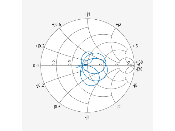
smithplot(freq,gIn);
drawnow

There are several ways to choose the cost function and some options are shown within the objective function above (in comments). The optimization variables are the first and last inductors, L1 and L5 respectively. The element values are stored in the variable L_Optimized.

niter = 125;
options = optimset('Display','iter','MaxIter',niter);  % Set options structure
L_Optimized = [Lvals(1) Lvals(end)];
L_Optimized = ...
    fminsearch(@(L_Optimized)antennaMatchObjectiveFun(matchingNW, ...
    L_Optimized,freq,Zl,Z0),L_Optimized,options);

 
 Iteration   Func-count         f(x)         Procedure
     0            1         0.933982         
     1            3         0.933982         initial simplex
     2            5         0.920323         expand
     3            7         0.911353         expand
     4            9         0.853255         expand
     5           11         0.730444         expand
     6           13         0.526448         reflect
     7           15         0.526448         contract inside
     8           17         0.421103         reflect
     9           19         0.421103         contract inside
    10           20         0.421103         reflect
    11           22         0.421103         contract inside
    12           24         0.421103         contract inside
    13           26         0.339935         expand
    14           27         0.339935         reflect
    15           29          0.28528         reflect
    16           31          0.28528         contract inside
    17           32          0.28528         reflect
    18           34         0.283527         reflect
    19           36         0.283527         contract inside
    20           38         0.278939         contract inside
    21           40         0.278123         reflect
    22           41         0.278123         reflect
    23           43          0.27636         contract inside
    24           45         0.275782         contract inside
    25           47         0.275637         contract inside
    26           49         0.275498         reflect
    27           51         0.275282         contract inside
    28           52         0.275282         reflect
    29           54         0.275282         contract inside
    30           56         0.275282         contract inside
 
Optimization terminated:
 the current x satisfies the termination criteria using OPTIONS.TolX of 1.000000e-04 
 and F(X) satisfies the convergence criteria using OPTIONS.TolFun of 1.000000e-04

Figure contains an axes object. The hidden axes object contains an object of type line.

Update Matching Network Elements with Optimal Values

When the optimization routine stops, the optimized element values are stored in L_Optimized. The following code updates the input and output matching network with these values.

matchingNW.Inductances(1) = L_Optimized(1);     % Update the matching network inductor L1
matchingNW.Inductances(end) = L_Optimized(end); % Update the matching network inductor L5

Analyze and Display Optimization Results

Compare and plot the input reflection coefficient of the matched and unmatched results.

S = sparameters(matchingNW,freq,Z0);
gIn = gammain(S,Zl);
smithplot(freq,[gIn transpose(GammaL)],'LegendLabels',...
    {'#Gamma in (Matched)','#Gamma in (Unmatched)'})

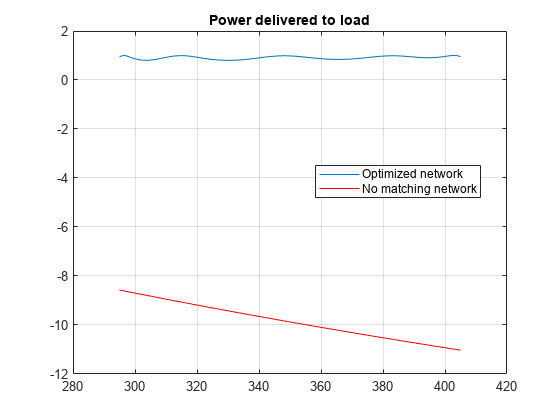
The optimized matching network improves the performance of the circuit. In the passband (295 - 405 MHz), the input reflection coefficient is closer to the center of the Smith chart. Plot the power delivered to load for both the matched and unmatched system.

matchedGt = powergain(S,Zs,Zl,'Gt');
figure;
plot(freq*1e-6,matchedGt)
hold on;
plot(freq*1e-6,unmatchedGt,'r')
grid on;
hold off;
title('Power delivered to load');
legend('Optimized network','No matching network','Location','Best');

Figure contains an axes object. The axes object with title Power delivered to load contains 2 objects of type line. These objects represent Optimized network, No matching network.

The power delivered to the load is approximately 1 dB down for the optimized matching network.

Display Optimized Element Values

The following code shows the initial and optimized values for inductors L1 and L5.

L1_Initial = L_initial(1)

L1_Initial = 
1.2340e-07

L1_Optimized = L_Optimized(1)

L1_Optimized = 
1.2111e-07

L5_Initial = L_initial(end)

L5_Initial = 
1.2340e-07

L5_Optimized = L_Optimized(end)

L5_Optimized = 
1.7557e-09

There are few things to consider when setting up an optimization:

Choosing a different objective function would change the result.
You can use advanced direct search optimization functions such as patternsearch and simulannealband in your optimization, but you must have the Global Optimization Toolbox™ installed to access them.

References

Cuthbert, Thomas R. Broadband Direct-Coupled and Matching RF Networks. TRCPEP, 1999.
Ludwig, Reinhold, and Pavel Bretchko. RF Circuit Design: Theory and Applications. Prentice-Hall, 2000.
Pozar, David. Microwave Engineering. 2nd ed., John Wiley and Sons, 1999.