Design, Visualize and Explore Inverse Chebyshev Filter - I

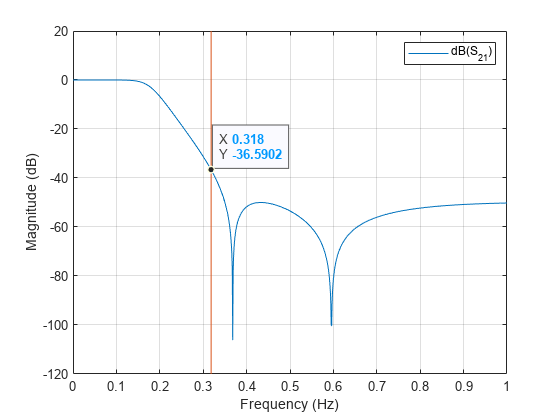
This example uses:

This example shows how to determine the transfer function for a fifth-order inverse Chebyshev lowpass filter with 1 dB passband attenuation, cutoff frequency of 1 rad/sec, and a minimum attenuation of 50 dB in the stopband. Determine the amplitude response at 2 rad/sec [1].

The rffilter object is used to design a RF Filter. A filter requires a minimum set of parameters for it to be completely defined. Refer to the table in the rffilter documentation page which reflects this set of required parameters. Each set of parameters result in its corresponding syntax. Input these parameters as name-value pairs to rffilter to design the specified filter. Note that the parameters which are required but are not defined assume default values.

After initialization of an rffilter object, the property DesignData contains the complete solution of the filter designed. It is a structure which contains fields such as the computed factorized polynomials for the construction of the transfer function.

Design Chebyshev Type II filter

N           = 5;            % Filter order
Fp          = 1/(2*pi);     % Passband cutoff frequency 
Ap          = 1;            % Passband attenuation
As          = 50;           % Stopband attenuation

Use rffilter object to create a desired filter. The only implementation type for Inverse Chebyshev is 'Transfer function'.

r = rffilter('FilterType','InverseChebyshev','ResponseType','Lowpass',  ...
    'Implementation','Transfer function','FilterOrder',N,               ...
    'PassbandFrequency',Fp,'StopbandAttenuation',As,                    ...
    'PassbandAttenuation',Ap);

Generate and Visualize Transfer Function Polynomial

Use tf function to generate transfer function polynomials.

[numerator, denominator] = tf(r);
format long g

Display Numerator21 polynomial coefficients.

disp('Numerator polynomial coefficients of Transfer function');

Numerator polynomial coefficients of Transfer function

disp(numerator{2,1});

        0.0347736250821381                         0         0.672768334081369                         0           2.6032214373595

Display Denominator polynomial coefficients.

disp('Denominator polynomial coefficients of Transfer function');

Denominator polynomial coefficients of Transfer function

disp(denominator);

                         1          3.81150884154936           7.2631952221038          8.61344575257214          6.42982763112227           2.6032214373595

Optionally, use Control System Toolbox™ to visualize all transfer functions.

G_s = tf(numerator,denominator)

G_s =
 
  From input 1 to output...
                                 s^5
   1:  --------------------------------------------------------
       s^5 + 3.812 s^4 + 7.263 s^3 + 8.613 s^2 + 6.43 s + 2.603
 
                   0.03477 s^4 + 0.6728 s^2 + 2.603
   2:  --------------------------------------------------------
       s^5 + 3.812 s^4 + 7.263 s^3 + 8.613 s^2 + 6.43 s + 2.603
 
  From input 2 to output...
                   0.03477 s^4 + 0.6728 s^2 + 2.603
   1:  --------------------------------------------------------
       s^5 + 3.812 s^4 + 7.263 s^3 + 8.613 s^2 + 6.43 s + 2.603
 
                                 s^5
   2:  --------------------------------------------------------
       s^5 + 3.812 s^4 + 7.263 s^3 + 8.613 s^2 + 6.43 s + 2.603
 
Continuous-time transfer function.

Visualize Amplitude Response of Filter

frequencies = linspace(0,1,1001);
Sparam      = sparameters(r, frequencies);

Note: S-parameters computes the transfer function using quadratic (lowpass/highpass) or quartic (bandpass/bandstop) factorized forms. These factors are used to construct the polynomials. The polynomial form is numerically unstable for larger filter order so the preferred form is the factorized quadratic/quartic forms. These factorized parts are present in r.DesignData. For example, the numerator21 can be accessed using r.DesignData.Numerator21.

l = rfplot(Sparam,2,1);

$Figure contains an axes object. The axes object with xlabel Frequency (Hz), ylabel Magnitude (dB) contains an object of type line. This object represents dB(S_{21}).$

Amplitude Response of Filter at Specified Frequency

freq     = 2/(2*pi);
hold on;
setrfplot('noengunits',false);

Note: To use rfplot and plot on the same figure use setrfplot.

plot(freq*ones(1,101),linspace(-120,20,101));
setrfplot('engunits',false);
[~,freq_index]= min(abs(frequencies-freq));
datatip(l,'DataIndex',freq_index);

$Figure contains an axes object. The axes object with xlabel Frequency (Hz), ylabel Magnitude (dB) contains 2 objects of type line. This object represents dB(S_{21}).$

Using the data tip, the magnitude at 2 rad/sec is found to be -36.59 dB.

Evaluate the exact value at 2 rad/sec.

S_freq   = sparameters(r,freq);
As_freq  = 20*log10(abs(rfparam(S_freq,2,1)));
sprintf('Amplitude response at 2 rad/sec is %d dB',As_freq)

ans = 
'Amplitude response at 2 rad/sec is -3.668925e+01 dB'

Calculate Stopband Frequency at As

Fs      = r.DesignData.Auxiliary.Wx*r.PassbandFrequency;
sprintf('Stopband frequency at -%d dB is: %d Hz',As, Fs)

ans = 
'Stopband frequency at -50 dB is: 3.500241e-01 Hz'

References

[1] Ellis, Michael G. Electronic Filter Analysis and Synthesis. Boston: Artech House, 1994.