Test, Visualize, and Enforce Passivity of Rational Output
This example shows how to test, visualize, and enforce the passivity of output from the rational function.
S-Parameter Data Passivity
Time-domain analysis and simulation depend critically on the ability to convert frequency-domain S-parameter data into causal, stable, and passive time-domain representations. Because the rational function guarantees that all poles are in the left half plane, rational output is both stable and causal by construction. The problem is passivity.
N-port S-parameter data represents a frequency-dependent transfer function H(f). You can create an S-parameters object in RF Toolbox™ by reading a Touchstone® file, such as passive.s2p, into the sparameters function.
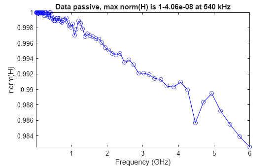
You can use the ispassive function to check the passivity of the S-parameter data, and the passivity function to plot the 2-norm of the N-by-N matrices H(f) at each data frequency.
S = sparameters('passive.s2p');
ispassive(S)
ans = logical
1
passivity(S)
Testing and Visualizing rational Output Passivity
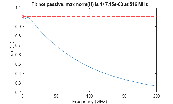
The rational function converts N-port S-parameter data, S, into an object that represents a rational fit to the data. Using the ispassive function on the output reports that even if input data S is passive, the output fit is not passive. In other words, the norm H(f) is greater than 1 at some frequency in the range [0,Inf].
The passivity function takes the output of the rational function as input and plots its passivity. This is a plot of the upper bound of the norm(H(f)) on [0,Inf], also known as the H-infinity norm.
fit = rational(S); ispassive(fit)
ans = logical
0
passivity(fit)
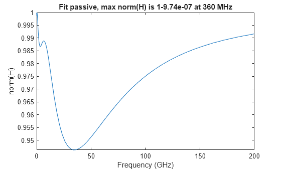
The makepassive function takes as input a rational object, and produces a passive fit by using convex optimization techniques to optimally match the data of the S-parameter input S while satisfying passivity constraints. The residues and direct term of the output pfit are modified, but the poles of the output pfit are identical to the poles of the input fit.
pfit = makepassive(fit,'Display','on');
Iter H-infinity norm Frequency Error (dB) Constraints 0 1+7.15e-03 516 MHz -40.4597 1 1+5.44e-04 319 MHz -41.755 5 2 1+7.80e-05 383 MHz -41.7319 7 3 1+8.60e-06 359 MHz -41.728 9 4 1-9.54e-07 360 MHz -41.7272 10
ispassive(pfit)
ans = logical
   1
passivity(pfit)
all(pfit.Poles == fit.Poles)
ans = logical
   1
Generate Equivalent SPICE Circuit from Passive Fit
The generateSPICE function takes a passive fit and generates an equivalent circuit as a SPICE subcircuit file. The input fit is an object as returned by rational with an S-parameters object as input. The generated file is a SPICE model constructed solely of passive R, L, C elements and controlled source elements E, F, G, and H.
generateSPICE(pfit,'mypassive.ckt')
type mypassive.ckt
* Equivalent circuit model for mypassive.ckt
.SUBCKT mypassive po1 po2
Vsp1 po1 p1 0
Vsr1 p1 pr1 0
Rp1 pr1 0 50
Ru1 u1 0 50
Fr1 u1 0 Vsr1 -1
Fu1 u1 0 Vsp1 -1
Ry1 y1 0 1
Gy1 p1 0 y1 0 -0.02
Vsp2 po2 p2 0
Vsr2 p2 pr2 0
Rp2 pr2 0 50
Ru2 u2 0 50
Fr2 u2 0 Vsr2 -1
Fu2 u2 0 Vsp2 -1
Ry2 y2 0 1
Gy2 p2 0 y2 0 -0.02
Rx1 x1 0 1
Fxc1_2 x1 0 Vx2 1.73984162430531
Cx1 x1 xm1 4.40797248385644e-09
Vx1 xm1 0 0
Gx1_1 x1 0 u1 0 -0.063779455862577
Rx2 x2 0 1
Fxc2_1 x2 0 Vx1 -1.10434591526148
Cx2 x2 xm2 4.40797248385644e-09
Vx2 xm2 0 0
Gx2_1 x2 0 u1 0 0.0704345815594368
Rx3 x3 0 1
Cx3 x3 0 2.46549192009636e-12
Gx3_1 x3 0 u1 0 -0.857325123346981
Rx4 x4 0 1
Cx4 x4 0 1.19630320666017e-11
Gx4_1 x4 0 u1 0 -2.76955836729716
Rx5 x5 0 1
Cx5 x5 0 1.85575917542297e-11
Gx5_1 x5 0 u1 0 -1.31131720743262
Rx6 x6 0 1
Cx6 x6 0 8.71015575148899e-11
Gx6_1 x6 0 u1 0 -0.691518069492981
Rx7 x7 0 1
Cx7 x7 0 5.76402178849075e-10
Gx7_1 x7 0 u1 0 -0.0721160728592211
Rx8 x8 0 1
Cx8 x8 0 1.32870599582361e-08
Gx8_1 x8 0 u1 0 -0.853447833732114
Rx9 x9 0 1
Fxc9_10 x9 0 Vx10 1.74900239748286
Cx9 x9 xm9 4.40797248385644e-09
Vx9 xm9 0 0
Gx9_2 x9 0 u2 0 -0.0646450984824799
Rx10 x10 0 1
Fxc10_9 x10 0 Vx9 -1.09856166793636
Cx10 x10 xm10 4.40797248385644e-09
Vx10 xm10 0 0
Gx10_2 x10 0 u2 0 0.0710166272128235
Rx11 x11 0 1
Cx11 x11 0 2.46549192009636e-12
Gx11_2 x11 0 u2 0 -0.902822009243767
Rx12 x12 0 1
Cx12 x12 0 1.19630320666017e-11
Gx12_2 x12 0 u2 0 -2.78932004722754
Rx13 x13 0 1
Cx13 x13 0 1.85575917542297e-11
Gx13_2 x13 0 u2 0 -1.32149568325976
Rx14 x14 0 1
Cx14 x14 0 8.71015575148899e-11
Gx14_2 x14 0 u2 0 -0.731808194657596
Rx15 x15 0 1
Cx15 x15 0 5.76402178849075e-10
Gx15_2 x15 0 u2 0 -0.0762186511523284
Rx16 x16 0 1
Cx16 x16 0 1.32870599582361e-08
Gx16_2 x16 0 u2 0 -0.853742802031904
Gyc1_1 y1 0 x1 0 -1
Gyc1_2 y1 0 x2 0 -1
Gyc1_3 y1 0 x3 0 -1
Gyc1_4 y1 0 x4 0 0.13385280727634
Gyc1_5 y1 0 x5 0 -0.577033771006121
Gyc1_6 y1 0 x6 0 -1
Gyc1_7 y1 0 x7 0 1
Gyc1_8 y1 0 x8 0 0.998921707090479
Gyc1_9 y1 0 x9 0 0.98121367810286
Gyc1_10 y1 0 x10 0 0.985302565498011
Gyc1_11 y1 0 x11 0 0.821262415944741
Gyc1_12 y1 0 x12 0 -1
Gyc1_13 y1 0 x13 0 1
Gyc1_14 y1 0 x14 0 0.920277646010057
Gyc1_15 y1 0 x15 0 -0.916612671131817
Gyc1_16 y1 0 x16 0 -1
Gyd1_1 y1 0 u1 0 0.9994400699278
Gyd1_2 y1 0 u2 0 -0.012502716946109
Gyc2_1 y2 0 x1 0 0.992672388157124
Gyc2_2 y2 0 x2 0 0.990300720812708
Gyc2_3 y2 0 x3 0 0.823747345686729
Gyc2_4 y2 0 x4 0 -1
Gyc2_5 y2 0 x5 0 1
Gyc2_6 y2 0 x6 0 0.97433414786269
Gyc2_7 y2 0 x7 0 -0.968731714311011
Gyc2_8 y2 0 x8 0 -1
Gyc2_9 y2 0 x9 0 -1
Gyc2_10 y2 0 x10 0 -1
Gyc2_11 y2 0 x11 0 -1
Gyc2_12 y2 0 x12 0 0.207570876153522
Gyc2_13 y2 0 x13 0 -0.668013976848524
Gyc2_14 y2 0 x14 0 -1
Gyc2_15 y2 0 x15 0 1
Gyc2_16 y2 0 x16 0 0.998684457058086
Gyd2_1 y2 0 u1 0 0.0127544276678894
Gyd2_2 y2 0 u2 0 0.99932594328929
.ENDS