Using Weight Parameter with rationalfit
This example shows how to use the Weight parameter to improve the quality of the output of rationalfit.
By default, the rationalfit function minimizes the absolute error between the data and the rational function, treating all data points equally. If you want to emphasize some of the data points more than the others, use the Weight parameter.
For example, If the magnitude of the input data has a large dynamic range, it is often useful to be more concerned with the relative error at each data point, rather than the absolute error at each data point, so that the data points with relatively smaller magnitudes are fit accurately. The common way to do this is to set the Weight parameter to 1./abs(data).
To put the example above in practice, follow the steps below.
Read in the SAW filter data contained in the file
sawfilter.s2p, and plot theS21data.Use the
rationalfitfunction to fit a rational function to theS21data, with theWeightparameter set to its default value, and visually compare the results to the original data.Use
rationalfitagain, this time specifying theWeightparameter to be1./abs(S21), and see if the result improves.
Read and Visualize Data
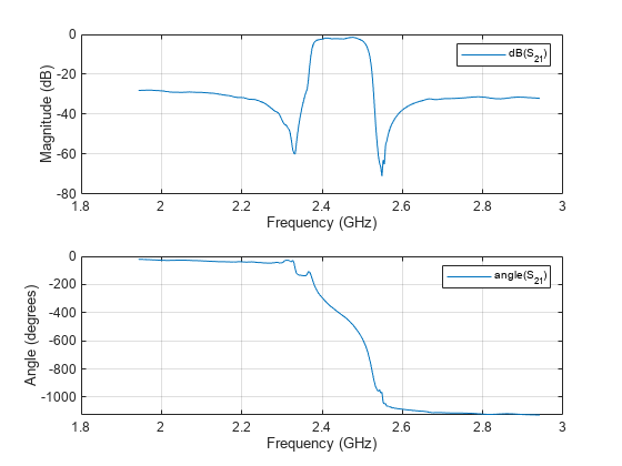
Read and visualize SAW filter S-parameters data.
S = sparameters('sawfilter.s2p');
figure
subplot(2,1,1)
rfplot(S,2,1,'db')
subplot(2,1,2)
rfplot(S,2,1,'angle')
Analyze Output of rationalfit When Using Default Value for Weight
Use the rfparam function to extract the S21 values, and then call rationalfit.
s21 = rfparam(S,2,1);
datafreq = S.Frequencies;
defaultfit = rationalfit(datafreq,s21);
Use the freqresp function to calculate the response of the output of rationalfit.
respfreq = 1e9:1.5e6:4e9;
defaultresp = freqresp(defaultfit,respfreq);
Compare the original data against the frequency response of the default rational function calculated by rationalfit.
subplot(2,1,1)
plot(datafreq,20*log10(abs(s21)),'.-')
hold on
plot(respfreq,20*log10(abs(defaultresp)))
hold off
xlabel("Frequency (Hz)")
ylabel("Magnitude (dB)")
defaultnpoles = numel(defaultfit.A);
defaultstr = ["Default Weight (Uses ",num2str(defaultnpoles)," poles)"];
title(defaultstr)
legend("Original Data","Default rationalfit",Location="best")
subplot(2,1,2)
plot(datafreq,unwrap(angle(s21))*180/pi,'.-')
hold on
plot(respfreq,unwrap(angle(defaultresp))*180/pi)
hold off
xlabel("Frequency (Hz)")
ylabel("Angle (degrees)")
legend("Original Data","Default rationalfit",Location="best")
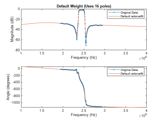
While the output of rationalfit is not awful, it does not match the regions in the data that are very small in magnitude.
figure
plot(datafreq,20*log10(abs(s21)),'.-')
hold on
plot(respfreq,20*log10(abs(defaultresp)))
hold off
axis([2.25e9 2.65e9 -75 -30])
xlabel("Frequency (Hz)")
ylabel("Magnitude (dB)")
title("Accuracy at Small Magnitudes Using Default Weight")
legend("Original Data","Default rationalfit",Location="best")
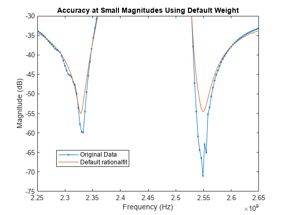
Using the Weight parameter to make that data relatively more important can help the accuracy of the fit.
Analyze Output of rationalfit When Using Custom Value for Weight
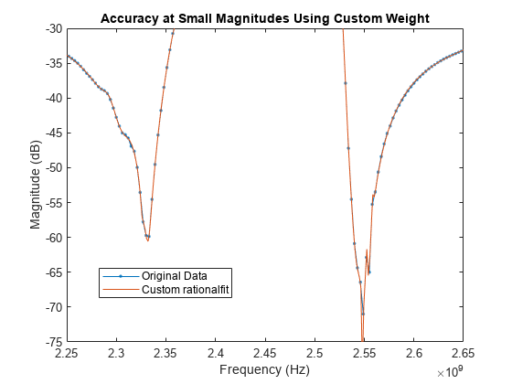
By using a Weight of 1./abs(s21), rationalfit minimizes the relative error of the system, instead of the absolute error of the system.
customfit = rationalfit(datafreq,s21,Weight=1./abs(s21));
Warning: Achieved only -39.7 dB accuracy with 48 poles, not -40.0 dB. Consider specifying a larger number of poles using the 'NPoles' parameter.
customresp = freqresp(customfit,respfreq);
Compare the original data against the frequency response of the custom rational function calculated by rationalfit.
figure
subplot(2,1,1)
plot(datafreq,20*log10(abs(s21)),'.-')
hold on
plot(respfreq,20*log10(abs(customresp)))
hold off
xlabel("Frequency (Hz)")
ylabel("Magnitude (dB)")
customnpoles = numel(customfit.A);
customstr = ["Weight = 1./abs(s21) (Uses ",num2str(customnpoles)," poles)"];
title(customstr)
legend("Original Data","Custom rationalfit",Location="best")
subplot(2,1,2)
plot(datafreq,unwrap(angle(s21))*180/pi,'.-')
hold on
plot(respfreq,unwrap(angle(customresp))*180/pi)
hold off
xlabel("Frequency (Hz)")
ylabel("Angle (degrees)")
legend("Original Data","Custom rationalfit",Location="best")
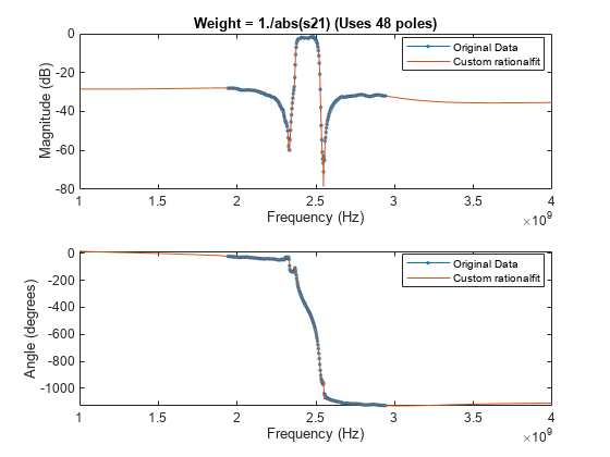
The plot shows that the custom Weight parameter created a better fit for the data points with smaller magnitudes.
figure
plot(datafreq,20*log10(abs(s21)),'.-')
hold on
plot(respfreq,20*log10(abs(customresp)))
hold off
axis([2.25e9 2.65e9 -75 -30])
xlabel("Frequency (Hz)")
ylabel("Magnitude (dB)")
title("Accuracy at Small Magnitudes Using Custom Weight")
legend("Original Data","Custom rationalfit",Location="best")
