Assess Climate Change Impact on Credit Risk Using UNEP FI Methodology

Open Live Script

This example shows a workflow based on the United Nations Environment Programme Finance Initiative (UNEP FI) methodology that you can use for assessing the potential impacts of climate change on corporate lending portfolios.

What Is the UNEP FI Methodology?

Linking financial impacts to credit outcomes is a key step in assessing the impact of climate change on credit risk. The methodology used in this workflow comes from a pilot program organized by UNEP FI [1], [4] and is useful for understanding this link. The Bank of Canada (BoC) used the UNEP FI methodology to conduct a scenario-based assessment of the potential impact of climate change on corporate lending portfolios. For more information about this assessment, see [2], [3], and [5].

The methodology requires an institution's experts to identify representative companies from each industry segment. The experts then assess the impact of a climate scenario on the companies’ credit ratings and probabilities of default (PD). The methodology uses a parametric model inspired by Merton's model for the PD shock. Using this model, you calibrate the PD shock to segment-level risk factor pathways (RFPs) consistent with the climate scenarios. You then use the expert-provided PD for the selected companies as a response. Once calibrated, you can use the model to shock the PD for any company.

The RFPs are direct emissions costs ( $c_{d}$ ), indirect costs ( $c_{i}$ ), capital expenditure ( $e_{c}$ ), and revenue ( $r$ ). You can calculate these quantities from the outputs of a climate scenario according to the following equations:

$c_{d} = p_{c} \times s$

$c_{i} = p_{i} \times N_{p}$

$e_{c} = p_{cap} \times n_{c}$

$r = p_{o} \times p$

where:

$p_{c}$ represents the carbon price.
$s$ represents the scope 1 emissions.
$p_{i}$ represents the input price.
$N_{p}$ represents the inputs in production.
$p_{cap}$ represents the capital price.
$n_{c}$ represents the new capital added.
$p_{o}$ represents the output price.
$p$ represents production.

For more details on these equations, see [5].

The RFPs combine into the following expression for net income ( $I_{n}$ ), which is expected to be negatively correlated with PD:

$I_{n} = r - c_{d} - c_{i} - e_{c}$

This workflow focuses on estimating the parameters you need to extrapolate expert-guided ratings to an entire portfolio. To estimate the required parameters, consider a borrower $i$ , in segment $j$ , within sector $k$ . Let $P D_{i, T T C}$ denote the through-the-cycle probability of default (PD) for borrower $i$ and $P D_{i, C}$ denote the scenario-adjusted PD for borrower $i$ . Assume that the quantity $P D_{i, C}$ has been provided by credit experts for a representative group of borrowers within each segment. Next, let $f_{k}^{r}$ represent $r$ risk factors that are allowed to depend on the sector $k$ . The workflow provides estimates for the scaling factor $α_{k}$ and the sensitivities $s_{j}^{r}$ in the main PD equation:

$P D_{i, C} = Φ [Φ^{- 1} (P D_{i, T T C}) - \frac{1}{α_{k}} \sum_{r} s_{j}^{r} f_{k}^{r}]$

where $Φ$ is the normal cumulative distribution function (CDF) and $Φ^{- 1}$ is the inverse CDF. The sum of risk factors and sensitivities is called the climate credit quality index. For more details about this index, see [1]. Once you estimate the scaling factor and sensitivities for the representative group of borrowers, you can use the same equation to score the general borrowers.

The methodology proposes using the Frye-Jacobs loss given default (LGD) model [6] to estimate a scenario-adjusted LGD from the through-the-cycle LGD, through-the-cycle PD, and scenario-adjusted PD. Together, the LGD and PD let you forecast the loss for each year covered by the climate scenarios. For information on computing the conditional LGD using the Frye-Jacobs function, see fryeJacobsLGD.

Process Climate Scenarios and Calibration Portfolio Data

The climate transition scenario data is provided by the Bank of Canada and is available free of charge at www.bankofcanada.ca [7].

After you load the BoC climate scenarios, remove unused variables, and rename the scenarios.

load("BankOfCanadaClimateScenarioData.mat");
climateData = renamevars(ClimateTransitionScenarioData, ...
    ["CL_GEOGRAPHY", "CL_SCENARIO", "CL_SECTOR", "CL_UNIT", "CL_VALUE", "CL_VARIABLE", "CL_YEAR"], ...
    ["Geography", "Scenario", "Sector", "Unit", "Value", "Variable", "Year"]);
climateData = removevars(climateData,["k","Unit"]);
climateData.Scenario = renamecats(climateData.Scenario, ...
    ["Baseline (2019 policies)", "Below 2°C delayed", "Below 2°C immediate", "Net-zero 2050 (1.5°C)"], ...
    ["Baseline", "Delayed", "Immediate", "NetZero"]);

The RFPs are the quantities that intervene in the methodology as shown in [1] and [2] and have already been computed for the BoC scenarios. Extract the RFPs from the climate data.

RFPs = ["Direct emissions costs", "Indirect costs", "Capital expenditure", "Revenue"];
idx = ismember(climateData.Variable, RFPs);
climateData = climateData(idx,:);
climateData = renamevars(climateData, "Variable", "RFP");
climateData.RFP = categorical(matlab.lang.makeValidName(string(climateData.RFP)));

Extract the US obligors which contains eleven sectors.

idx = climateData.Geography == "United States";
climateData = climateData(idx,:);
unique(climateData.Sector)

ans = 11×1 categorical
     Coal 
     Commercial transportation 
     Crops 
     Electricity 
     Energy-intensive industries 
     Forestry 
     Gas 
     Livestock 
     Oil 
     Oil & Gas 
     Refined oil products

The BoC implementation uses nine sectors that include the joint Oil & Gas sector, but exclude the individual Oil and Gas sectors.

sectors = ["Coal", "Commercial transportation", "Crops", "Electricity", "Energy-intensive industries", ...
    "Forestry", "Livestock", "Oil & Gas", "Refined oil products"];
idx = ismember(climateData.Sector, sectors);
climateData = climateData(idx,:);

Unstack the climate scenario data and store the data in separate columns.

climateData = unstack(climateData, "Value", "Scenario");

The RFPs enter the model as percent differences measured from the Baseline scenario.

climateData{:, ["BaselineRaw", "DelayedRaw", "ImmediateRaw", "NetZeroRaw"]} = ...
    climateData{:, ["Baseline", "Delayed", "Immediate", "NetZero"]};
climateData{:, ["Baseline", "Delayed", "Immediate", "NetZero"]} = ...
    (climateData{:, ["Baseline", "Delayed", "Immediate", "NetZero"]} - climateData{:, "Baseline"}) ./ climateData{:, "Baseline"};

Unstack the RFPs into separate columns for subsequent joining steps. Notice that the Indirect costs variable is missing for the Electricity sector.

climateDataJoin = unstack(climateData, ["Baseline", "Delayed", "Immediate", "NetZero", "BaselineRaw", "DelayedRaw", "ImmediateRaw", "NetZeroRaw"], "RFP");

When comparing the Sector column in this table with the sectors presented in the heatmap in [4], you can see that the sectors are not identical. However, since the Indirect Emissions Costs for Power Generation are similar to those of Transportation and Agriculture, you can use the Commercial transportation and Crops sectors from the BoC table as proxies for Indirect costs for the Electricity sector.

electricityIdx = climateDataJoin.Sector == "Electricity";
proxyIdx = climateDataJoin.Sector == "Commercial transportation" | climateDataJoin.Sector == "Crops";
indirectCostVars = climateDataJoin.Properties.VariableNames(contains(climateDataJoin.Properties.VariableNames, "Indirect"));
proxyTable = groupsummary(climateDataJoin(proxyIdx, :), "Year", "mean", indirectCostVars);
proxyValues = proxyTable{:, 3:10};
climateDataJoin{electricityIdx, indirectCostVars} = proxyValues;

Combine the RFPs into an expression for net income $I_{n}$ that you use when aggregating results.

scenarios = ["Baseline", "Delayed", "Immediate", "NetZero"];
factors = ["Revenue", "DirectEmissionsCosts", "IndirectCosts", "CapitalExpenditure"];
rawFactors = cell(1, numel(factors));

for i = 1:numel(factors)
    rawFactors{i} = strcat(scenarios, "Raw_", factors(i));
end

rawNetIncomeNames = strcat(scenarios, "Raw_", "NetIncome");
climateDataJoin{:, rawNetIncomeNames} = ...
    climateDataJoin{:, rawFactors{1}} - climateDataJoin{:, rawFactors{2}} - climateDataJoin{:, rawFactors{3}} - climateDataJoin{:, rawFactors{4}};

netIncomeNames = strcat(scenarios, "NetIncome");
climateDataJoin{:, netIncomeNames} = ...
    (climateDataJoin{:, rawNetIncomeNames} - climateDataJoin{:, "BaselineRaw_NetIncome"}) ./ climateDataJoin{:, "BaselineRaw_NetIncome"};

The calibration portfolio must be prepared by the institution's credit risk experts. It consists of representative exposures for each sector and segment with additional information required to calibrate the model. For this example, prepare a basic calibration portfolio with the following columns:

LoanID – Identification number of the loan.
Sector – Industry sector. Internal experts must provide a mapping from their exposures to an appropriate industry sector.
Segment – Industry segment. Internal experts must provide a mapping from their exposures to an appropriate industry segment.
ttcRating – Through-the-cycle rating for each exposure. This rating is generally provided by an internal model or vendor ratings and it is independent of any particular economic or climate scenario. It does not depend on the year.
immediateRatingExpert – Internal experts analyze the selected representative exposures and provide a rating conditioned on a given climate scenario. This example assumes that the experts have provided the forecasted rating for two years, 2035 and 2050, conditioned on the Immediate climate scenario. In practice, experts should provide ratings for as many years as is feasible. You can also try this workflow with other nonbaseline scenarios.
ttcPD – PD values corresponding to ttcRating. These values are generally provided by an internal mapping table between ratings and PD values. The matfile pdMappingTable.mat contains an example table.
immediatePDExpert – PD values corresponding to immediateRatingExpert. These values are generally provided by an internal mapping table between ratings and PD values. The matfile pdMappingTable.mat contains an example table.
Year – The year for which the expert has provided the conditional rating, (see the description for immediateRatingExpert).

In practice, the calibration portfolio includes at least these columns.

Load the calibration portfolio.

load("portfoliosUNEPFI.mat");

Join the climate data to the loan calibration portfolio.

calibrationPortfolioClimateData = join(calibrationPortfolio, climateDataJoin, "Keys", ["Sector", "Year"], "KeepOneCopy", ["Sector", "Year"]);

Fit the Parameters $α$ and $β$

Recall the main PD equation:

$P D_{i, C} = Φ [Φ^{- 1} (P D_{i, T T C}) - \frac{1}{α_{k}} \sum_{r} s_{j}^{r} f_{k}^{r}]$

The BoC paper, in fact, fits the following PD equation:

$P D_{i, C} = Φ [Φ^{- 1} (P D_{i, T T C}) - \frac{1}{α_{k}} (\sum_{r} s_{j}^{r} f_{k}^{r} - β_{k} {(\sum_{r} s_{j}^{r} f_{k}^{r})}^{2})]$

For each sector $k$ , you fit a scaling factor $α_{k}$ . The factor brings the climate credit quality index expressing the climate scenarios into the expected range and controls the magnitude of the sector-level relationship to the RFPs. The parameter $β_{k}$ is similar, but it accounts for nonlinear combinations of RFPs. For more details, see [2].

Recall that the response variable is the scenario-adjusted PD conditional on the Immediate scenario. To fit $α_{k}$ and $β_{k}$ , assume that the sensitivities $s_{j}^{r}$ are all equal to 1. Then, compute the climate credit quality index in the main PD equation using the values from the Immediate scenario.

The normalization of $α_{k}$ and $β_{k}$ in this example differs slightly from the BoC implementation. Instead, this example uses the following main PD equation:

$P D_{i, C} = Φ [Φ^{- 1} (P D_{i, T T C}) + α_{k} \sum_{r} s_{j}^{r} f_{k}^{r} + β_{k} {(\sum_{r} s_{j}^{r} f_{k}^{r})}^{2}]$

Calculate the climate credit quality index, assuming that the sensitivities are all equal to 1.

immediateRFPs = ["Immediate_CapitalExpenditure", "Immediate_DirectEmissionsCosts", "Immediate_IndirectCosts", "Immediate_Revenue"];
calibrationPortfolioClimateData.ImmediateRFPSum = sum(calibrationPortfolioClimateData{:, immediateRFPs}, 2);

Create a dictionary to store the parameters.

alphaDict = dictionary;
betaDict = dictionary;

Estimate the parameters for each sector. Apply a lower bound of 0 for both $α$ and $β$ in order to assume that these sectors are adversely affected by changes to the economy due to climate policies.

sectors = unique(calibrationPortfolioClimateData.Sector);
options = optimoptions("lsqnonlin", "Display", "off");

for i = 1:numel(sectors)
    sector = sectors(i);
    idx = calibrationPortfolioClimateData.Sector == sector;
    sectorData = calibrationPortfolioClimateData(idx, :);
    ttcPD = sectorData.ttcPD;
    stressedPD = sectorData.immediatePDExpert;
    immediateRFPSum = sectorData.ImmediateRFPSum;
    immediateRFPSumSquared = immediateRFPSum .* immediateRFPSum;

    fun = @(x) normcdf(norminv(ttcPD) + x(1) * immediateRFPSum + x(2) * immediateRFPSumSquared) - stressedPD;
    est = lsqnonlin(fun, [0, 0], [0, 0], [], options);

    alpha = est(1);
    beta = est(2);

    alphaDict(sector) = alpha;
    betaDict(sector) = beta;
end

Save the parameters in a table and treat small values as 0.

alphaTable = renamevars(entries(alphaDict),["Key", "Value"], ["Sector", "alpha"]);
betaTable = renamevars(entries(betaDict), ["Key", "Value"], ["Sector", "beta"]);
alphaBetaTable = join(alphaTable, betaTable, "KeepOneCopy", "Sector");
threshold = 1e-4;
alphaBetaTable.alpha(alphaBetaTable.alpha < threshold) = 0;
alphaBetaTable.beta(alphaBetaTable.beta < threshold) = 0;

Fit the Sensitivities

Next, fit the sensitivities at the segment level relative to the sector. To perform the fitting, the methodology utilizes sectoral segmentation and a heat map tool to evaluate the financial sensitivity of a given segment to the sectoral RFP components. This tool contains six qualitative levels: negative, low, moderately low, moderate, moderately high, and high. For more details, including a listing of segments within each sector and the qualitative sensitivities for each RFP, see [2].

In practice, you adjust the bounds according to expert judgment and the financial institution's internal data. Within each segment, coefficients with the same qualitative sensitivity are required to have the same estimated sensitivity. The qualitative sensitivities map to bounds according to the following table:

Sensitivity Bounds

Sensitivity Level	Lower Bound	Upper Bound
Low	0.1	0.5
Moderately low	0.5	1
Moderate	1	1
Moderately high	1	1.5
High	1.5	10
Negative	-2	-0.1

Next, create a dictionary to store the sensitivities.

sensitivitiesDict = dictionary;

For sectors with only one segment, all sensitivities are 1 by definition:

oneSegment = ["Livestock", "Forestry", "Crops", "Coal", "Refined oil products"];
for i = 1:numel(oneSegment)
    sector = oneSegment(i);
    sensitivitiesDict{sector} = [1, 1, 1, 1];
end

Estimate the sensitivities for the remaining segments.

remainingSegments = setdiff(string(unique(calibrationPortfolioClimateData.Segment)), oneSegment);

Use a dictionary to store the upper and lower bounds for each segment by accessing the sectoral segmentation and heat map tool in [2] together with the Sensitivity Bounds table.

lowerBounds = dictionary;
upperBounds = dictionary;

lowerBounds{"Oil and gas extraction (except oil sands)"} = [1, 0.5, 1, 1];
upperBounds{"Oil and gas extraction (except oil sands)"} = [1.5, 1, 1, 1];

lowerBounds{"Oil sands extraction"} = [1.5, 1, 1, 1.5];
upperBounds{"Oil sands extraction"} = [10, 1.5, 1.5, 10];

lowerBounds{"Crude petroleum from oil shale"} = [1, 1, 1, 1];
upperBounds{"Crude petroleum from oil shale"} = [1.5, 1.5, 1.5, 1.5];

lowerBounds{"Contract drilling and services to oil and gas extraction"} = [0.5, 1, 0.5, 1];
upperBounds{"Contract drilling and services to oil and gas extraction"} = [1, 1, 1, 1.5];

lowerBounds{"Pipeline transportation"} = [1, 1, 1, 0.5];
upperBounds{"Pipeline transportation"} = [1, 1.5, 1, 1];

lowerBounds{"Natural gas distribution"} = [0.1, 0.1, 0.5, 0.5];
upperBounds{"Natural gas distribution"} = [0.5, 0.5, 1, 1];

lowerBounds{"Fossil-fuel electric power generation"} = [1, 1, 1, -2];
upperBounds{"Fossil-fuel electric power generation"} = [1.5, 1.5, 1.5, -0.1];

lowerBounds{"Hydro and nuclear"} = [0.1, 0.1, 0.5, 0.5];
upperBounds{"Hydro and nuclear"} = [0.5, 0.5, 1, 1];

lowerBounds{"Other renewables"} = [0.1, 0.5, 0.5, 1];
upperBounds{"Other renewables"} = [0.5, 1, 1, 1.5];

lowerBounds{"Electric power transmission, control and distribution"} = [0.1, 0.1, 1, 1];
upperBounds{"Electric power transmission, control and distribution"} = [0.5, 0.5, 1, 1];

lowerBounds{"Paper manufacturing, printing and related support activities"} = [1, 0.5, 1, 1];
upperBounds{"Paper manufacturing, printing and related support activities"} = [1.5, 1, 1, 1];

lowerBounds{"Chemical manufacturing, plastics and rubber products manufacturing"} = [1, 0.5, 1, 1];
upperBounds{"Chemical manufacturing, plastics and rubber products manufacturing"} = [1, 1, 1.5, 1];

lowerBounds{"Non-metallic mineral product manufacturing"} = [1, 1, 0.5, 1];
upperBounds{"Non-metallic mineral product manufacturing"} = [1.5, 1, 1, 1];

lowerBounds{"Primary metal manufacturing and fabricated metal product manufacturing"} = [0.5, 1.5, 1.5, 1];
upperBounds{"Primary metal manufacturing and fabricated metal product manufacturing"} = [1, 10, 10, 1];

lowerBounds{"Air transportation"} = [1.5, 0.5, 1.5, 0.1];
upperBounds{"Air transportation"} = [10, 1, 10, 0.5];

lowerBounds{"Rail transportation"} = [0.5, 0.1, 0.5, 1];
upperBounds{"Rail transportation"} = [1, 0.5, 1, 1.5];

lowerBounds{"Water transportation"} = [1, 0.5, 1, 1];
upperBounds{"Water transportation"} = [1.5, 1, 1.5, 1];

lowerBounds{"Other transportation"} = [0.5, 1.5, 1, 1];
upperBounds{"Other transportation"} = [1, 10, 1, 1];

Read the linear equalities between coefficients determined by the heat map and store them in a dictionary.

AeqDict = dictionary;
BeqDict = dictionary;

AeqDict{"Oil and gas extraction (except oil sands)"} = [];
BeqDict{"Oil and gas extraction (except oil sands)"} = [];

AeqDict{"Oil sands extraction"} = [1, 0, 0, -1; 0, 1, -1, 0];
BeqDict{"Oil sands extraction"} = [0; 0];

AeqDict{"Crude petroleum from oil shale"} = [1, -1, 0, 0; 1, 0, -1, 0; 1, 0, 0, -1];
BeqDict{"Crude petroleum from oil shale"} = [0; 0; 0];

AeqDict{"Contract drilling and services to oil and gas extraction"} = [1, 0, -1, 0];
BeqDict{"Contract drilling and services to oil and gas extraction"} = 0;

AeqDict{"Pipeline transportation"} = [];
BeqDict{"Pipeline transportation"} = [];

AeqDict{"Natural gas distribution"} = [1, -1, 0, 0; 0, 0, 1, -1];
BeqDict{"Natural gas distribution"} = [0; 0];

AeqDict{"Fossil-fuel electric power generation"} = [1, -1, 0, 0; 1, 0, -1, 0];
BeqDict{"Fossil-fuel electric power generation"} = [0; 0];

AeqDict{"Hydro and nuclear"} = [1, -1, 0, 0; 0, 0, 1, -1];
BeqDict{"Hydro and nuclear"} = [0; 0];

AeqDict{"Other renewables"} = [0, 1, -1, 0];
BeqDict{"Other renewables"} = 0;

AeqDict{"Electric power transmission, control and distribution"} = [1, -1, 0, 0];
BeqDict{"Electric power transmission, control and distribution"} = 0;

AeqDict{"Paper manufacturing, printing and related support activities"} = [];
BeqDict{"Paper manufacturing, printing and related support activities"} = [];

AeqDict{"Chemical manufacturing, plastics and rubber products manufacturing"} = [];
BeqDict{"Chemical manufacturing, plastics and rubber products manufacturing"} = [];

AeqDict{"Non-metallic mineral product manufacturing"} = [];
BeqDict{"Non-metallic mineral product manufacturing"} = [];

AeqDict{"Primary metal manufacturing and fabricated metal product manufacturing"} = [0, 1, -1, 0];
BeqDict{"Primary metal manufacturing and fabricated metal product manufacturing"} = 0;

AeqDict{"Air transportation"} = [1, 0, -1, 0];
BeqDict{"Air transportation"} = 0;

AeqDict{"Rail transportation"} = [1, 0, -1, 0];
BeqDict{"Rail transportation"} = 0;

AeqDict{"Water transportation"} = [1, 0, -1, 0];
BeqDict{"Water transportation"} = 0;

AeqDict{"Other transportation"} = [];
BeqDict{"Other transportation"} = [];

Use least-squares optimization to estimate the sensitivities for the remaining segments. Recall that the expert PD was assumed to apply to the Immediate scenario.

for i = 1:numel(remainingSegments)
    segment = remainingSegments(i);
    idx = calibrationPortfolioClimateData.Segment == segment;
    segmentData = calibrationPortfolioClimateData(idx, :);
    sector = unique(segmentData.Sector);
    ttcPD = segmentData.ttcPD;
    stressedPD = segmentData.immediatePDExpert;
    directEmissionsCosts = segmentData.Immediate_DirectEmissionsCosts;
    indirectCosts = segmentData.Immediate_IndirectCosts;
    capitalExpenditure = segmentData.Immediate_CapitalExpenditure;
    revenue = segmentData.Immediate_Revenue;
    alpha = alphaBetaTable{alphaBetaTable.Sector == sector, "alpha"};
    beta = alphaBetaTable{alphaBetaTable.Sector == sector, "beta"};

    fun = @(s) normcdf(norminv(ttcPD) ...
        + alpha*(s(1)*directEmissionsCosts + s(2)*indirectCosts + s(3)*capitalExpenditure + s(4)*revenue) ...
        + beta*(s(1)*directEmissionsCosts + s(2)*indirectCosts + s(3)*capitalExpenditure + s(4)*revenue).^2) ...
        - stressedPD;
    s0 = [1, 1, 1, 1];
    lb = lowerBounds{segment};
    ub = upperBounds{segment};
    A = [];
    b = [];
    Aeq = AeqDict{segment};
    Beq = BeqDict{segment};
    sensitivities = lsqnonlin(fun,s0,lb,ub,A,b,Aeq,Beq,[],options);

    sensitivitiesDict{segment} = sensitivities;
end

Save the sensitivities in a table.

sensitivitiesTable = entries(sensitivitiesDict);
sensitivitiesTable{:,3:6} = cell2mat(sensitivitiesTable.Value);
sensitivitiesTable = removevars(sensitivitiesTable,"Value");
sensitivitiesTable = renamevars(sensitivitiesTable,{'Key','Var3','Var4','Var5','Var6'},{'Segment','sDirectEmissionsCosts','sIndirectCosts','sCapitalExpenditure','sRevenue'});
sensitivitiesTable.Segment = categorical(sensitivitiesTable.Segment);

Validate the Model

Now that the parameters have been calibrated, you can validate the model against the expert credit ratings.

Attach the parameters to the calibration portfolio.

calibrationPortfolioClimateData = join(calibrationPortfolioClimateData, alphaBetaTable);
calibrationPortfolioClimateData = join(calibrationPortfolioClimateData, sensitivitiesTable);

Use the model to predict PD in the Immediate scenario by using the main PD equation. Then, use the PD mapping table to map the predicted PD to a predicted rating.

ttcPD = calibrationPortfolioClimateData.ttcPD;
alpha = calibrationPortfolioClimateData.alpha;
beta = calibrationPortfolioClimateData.beta;
sensitivities = [calibrationPortfolioClimateData.sDirectEmissionsCosts, ...
    calibrationPortfolioClimateData.sIndirectCosts, ...
    calibrationPortfolioClimateData.sCapitalExpenditure, calibrationPortfolioClimateData.sRevenue];

load("pdMappingTable.mat", "pdMappingTable");
edges = [0; pdMappingTable.PD];

RFPs = [calibrationPortfolioClimateData.("Immediate_DirectEmissionsCosts"), ...
    calibrationPortfolioClimateData.("Immediate_IndirectCosts"), ...
    calibrationPortfolioClimateData.("Immediate_CapitalExpenditure"), ...
    calibrationPortfolioClimateData.("Immediate_Revenue")];
climateCreditQualityIndex = sum(sensitivities .* RFPs, 2);
climateCreditQualityIndexSquared = climateCreditQualityIndex.^2;
calibrationPortfolioClimateData.("immediatePDPredicted") = normcdf(norminv(ttcPD) + alpha .* climateCreditQualityIndex + beta .* climateCreditQualityIndexSquared);
calibrationPortfolioClimateData.("immediateRatingPredicted") = discretize(calibrationPortfolioClimateData.("immediatePDPredicted"), edges);

Create a confusion chart to compare the expert and predicted ratings.

confusionchart(calibrationPortfolioClimateData.immediateRatingExpert, calibrationPortfolioClimateData.immediateRatingPredicted)
title("Confusion Chart")

Figure contains an object of type ConfusionMatrixChart. The chart of type ConfusionMatrixChart has title Confusion Chart.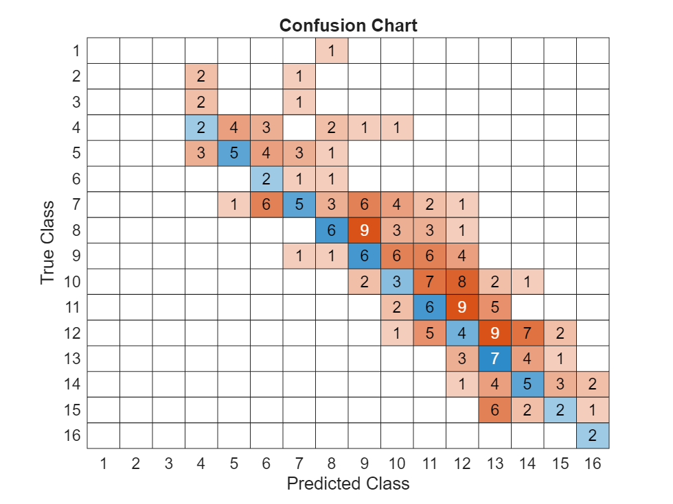

The calibrated model appears to be overly conservative compared to the experts ratings. For stress testing applications, a conservative approach is generally considered appropriate. If you want to make a model more accurate, you might need to adjust the bounds on the sensitivities or consult the credit risk experts who generated the calibration data.

Score a Portfolio

In the previous section, you used the model to score the calibration data. One purpose of the methodology is to extrapolate the expert ratings provided for a group of representative borrowers to an entire portfolio. In this section, you score the entire portfolio for all years covered by the scenarios.

To score a portfolio, you need only these variables: Sector, Segment, and through-the-cycle rating. Next, display the first eight rows of a portfolio to observe these variables. As noted earlier, institutions generally have an internal mapping table to go between ratings and PDs. Use the mapping table to attach the PD corresponding to the through-the-cycle rating to each loan.

fullPortfolio = join(fullPortfolio, pdMappingTable, "LeftKeys", "ttcRating", "RightKeys", "NumericRating", "RightVariables", "PD");
fullPortfolio = renamevars(fullPortfolio, "PD", "ttcPD");

The parameters were estimated using the calibration portfolio. Attach the parameters to the full portfolio.

fullPortfolio = join(fullPortfolio, alphaBetaTable);
fullPortfolio = join(fullPortfolio, sensitivitiesTable);

The scenarios cover the period 2020 through 2050 in 5 year increments. Expand the data into a panel data set with one observation for each LoanID in each year.

c = cell(7, 1);
for year = 2020:5:2050
    t = [fullPortfolio, array2table(repmat(year, height(fullPortfolio), 1), "VariableNames", "Year")];
    c{(year - 2020) / 5 + 1} = t;
end
fullPortfolioPanel = vertcat(c{:});
fullPortfolioPanel = sortrows(fullPortfolioPanel, ["LoanID", "Year"]);

Attach the RFPs from the climate data, which are based on Sector and Year.

fullPortfolioPanel = join(fullPortfolioPanel, climateDataJoin, "RightVariables",["Delayed_CapitalExpenditure", "Delayed_DirectEmissionsCosts", ... 
    "Delayed_IndirectCosts", "Delayed_Revenue", "Immediate_CapitalExpenditure", ... 
    "Immediate_DirectEmissionsCosts", "Immediate_IndirectCosts", ... 
    "Immediate_Revenue", "NetZero_CapitalExpenditure", ... 
    "NetZero_DirectEmissionsCosts", "NetZero_IndirectCosts", "NetZero_Revenue"]);

Use the calibrated parameters to predict PD for each observation in the nonbaseline scenarios. Then, map the predicted PD to a predicted rating using the PD mapping table.

ttcPD = fullPortfolioPanel.ttcPD;
alpha = fullPortfolioPanel.alpha;
beta = fullPortfolioPanel.beta;
sensitivities = table2array(fullPortfolioPanel(:, ["sDirectEmissionsCosts", "sIndirectCosts", "sCapitalExpenditure", "sRevenue"]));

nonBaselineScenarios = ["Delayed", "Immediate", "NetZero"];
edges = [0; pdMappingTable.PD];

for i = 1:numel(nonBaselineScenarios)
    scenario = nonBaselineScenarios(i);
    RFPNames = scenario + "_" + ["DirectEmissionsCosts", "IndirectCosts", "CapitalExpenditure", "Revenue"]; 
    RFPs = table2array(fullPortfolioPanel(:, RFPNames));
    climateCreditQualityIndex = sum(sensitivities .* RFPs, 2);
    climateCreditQualityIndexSquared = climateCreditQualityIndex.^2;
    fullPortfolioPanel.(strcat(lower(scenario), "PDPredicted")) = normcdf(norminv(ttcPD) + alpha .* climateCreditQualityIndex + beta .* climateCreditQualityIndexSquared);
    fullPortfolioPanel.(strcat(lower(scenario), "RatingPredicted")) = discretize(fullPortfolioPanel.(strcat(lower(scenario), "PDPredicted")), edges);
end

Finally, attach the expert ratings from the calibration portfolio. Only those observations in the full portfolio panel data corresponding to observations in the calibration portfolio have expert ratings. Specifically, these observations are for loan IDs 1 through 115 in years 2035 and 2050.

fullPortfolioPanel = outerjoin(fullPortfolioPanel, calibrationPortfolio, ...
    "Keys", ["LoanID", "Year"], ...
    "RightVariables", ["immediateRatingExpert", "immediatePDExpert"]);

Predict LGD

Both the climate-adjusted PD and LGD are required to compute the climate-adjusted loss. The methodology proposes using the Frye-Jacobs function to estimate the scenario-adjusted LGD.

Assume a 30% through-the-cycle LGD rate and use the climate-adjusted PD to calculate a climate-adjusted conditional LGD using the fryeJacobsLGD function.

fullPortfolioPanel.ttcLGD = repmat(.30, height(fullPortfolioPanel), 1);
ttcLGD = fullPortfolioPanel.ttcLGD;
ttcPD = fullPortfolioPanel.ttcPD;

for i = 1:numel(scenarios)
    scenario = lower(scenarios(i));
    if scenario ~= "baseline"
        adjustedPD = fullPortfolioPanel.(strcat(scenario, "PDPredicted"));
        fullPortfolioPanel.(strcat(scenario, "LGDPredicted")) = fryeJacobsLGD(adjustedPD, ttcPD, ttcLGD, 0);
    end
end

Additionally, use the expert PD to calculate an expert LGD for the observations in the calibration portfolio.

fullPortfolioPanel.immediateLGDExpert = fryeJacobsLGD(fullPortfolioPanel.immediatePDExpert, ttcPD, ttcLGD, 0);

Compute Losses and Aggregate Results

Now that you have obtained the climate-adjusted PD and LGD, you can compute the climate-adjusted expected loss rate (ELR) using this formula:

$ELR = PD x LGD$

If you have an estimate for the EAD, you can compute the expected loss (EL) using this formula:

$EL = PD x LGD x EAD$

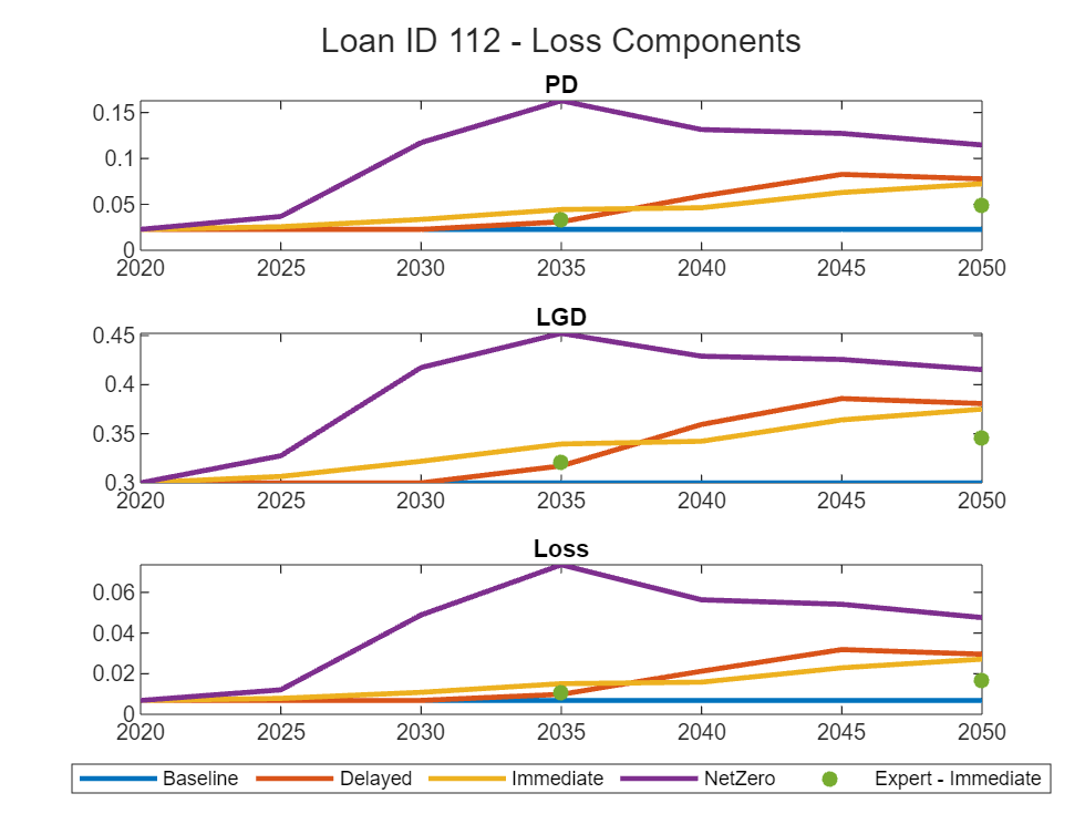
You can plot the PD, LGD, and EL against time for a single obligor [2]. To make these plots, first calculate the loss estimates using the formula above. The expert predicted loss is available only for the observations corresponding to the calibration portfolio.

fullPortfolioPanel{:, ["ttcLoss", "delayedLossPredicted", "immediateLossPredicted", "netzeroLossPredicted", "immediateLossExpert"]} = ... 
    fullPortfolioPanel{:, ["ttcPD", "delayedPDPredicted", "immediatePDPredicted", "netzeroPDPredicted", "immediatePDExpert"]} ... 
    .* fullPortfolioPanel{:, ["ttcLGD", "delayedLGDPredicted", "immediateLGDPredicted", "netzeroLGDPredicted", "immediateLGDExpert"]};

Plot the results. The points representing the expert prediction are available only for the loans in the calibration portfolio. You can choose any loan ID from 1 to 115.

lossComponents = ["PD", "LGD", "Loss"];
years = 2020:5:2050;

LoanID = 112;
idx = fullPortfolioPanel.LoanID == LoanID;
loanPortfolioData = fullPortfolioPanel(idx, :);
idx = fullPortfolioPanel.LoanID == LoanID;
loanBacktestData = fullPortfolioPanel(idx, :);

figure;
tlo = tiledlayout(3, 1);
title(tlo, strcat("Loan ID ", string(LoanID), " - Loss Components"));

for i = 1:numel(lossComponents)
    lossComponent = lossComponents(i);
    nexttile;
    
    plot(years, loanPortfolioData.(strcat("ttc", lossComponent)), 'LineWidth', 2);
    hold on;
    plot(years, loanPortfolioData.(strcat("delayed", lossComponent, "Predicted")), 'LineWidth', 2);
    plot(years, loanPortfolioData.(strcat("immediate", lossComponent, "Predicted")), 'LineWidth', 2);
    plot(years, loanPortfolioData.(strcat("netzero", lossComponent, "Predicted")), 'LineWidth', 2);
    
    scatter(loanBacktestData.Year, loanBacktestData.(strcat("immediate", lossComponent, "Expert")), 'filled');
    
    hold off;
    title(lossComponent);
end

lg = legend("Baseline", "Delayed", "Immediate", "NetZero", "Expert - Immediate", ...
            'Orientation', 'Horizontal', 'NumColumns', 5);
lg.Layout.Tile = 'South';

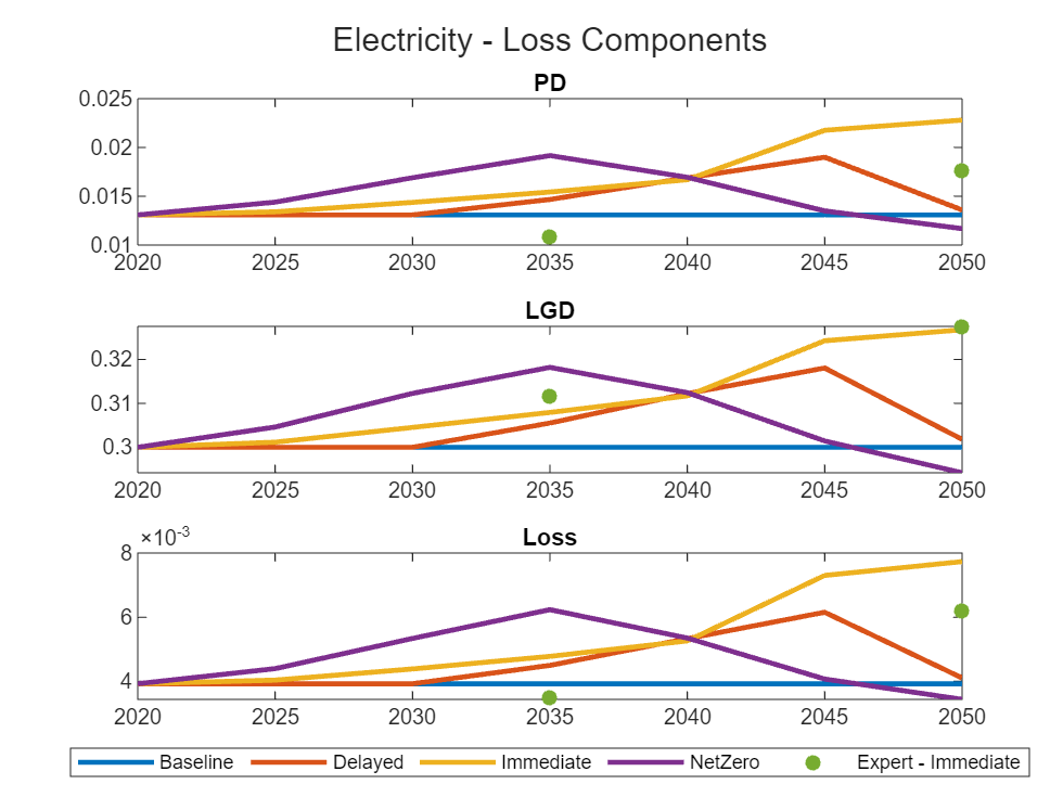
Figure contains 3 axes objects. Axes object 1 with title PD contains 5 objects of type line, scatter. Axes object 2 with title LGD contains 5 objects of type line, scatter. Axes object 3 with title Loss contains 5 objects of type line, scatter. These objects represent Baseline, Delayed, Immediate, NetZero, Expert - Immediate.

You can also create loss component plots at the sector level.

sectorPortfolioSummary = groupsummary(fullPortfolioPanel, ["Sector", "Year"], "mean", ... 
["ttcPD", "delayedPDPredicted", "immediatePDPredicted", "netzeroPDPredicted", ... 
"ttcLGD", "delayedLGDPredicted", "immediateLGDPredicted", "netzeroLGDPredicted", ...
"ttcLoss", "delayedLossPredicted", "immediateLossPredicted", "netzeroLossPredicted"]);

idx = ~isnan(fullPortfolioPanel.immediatePDExpert);
sectorCalibrationSummary = groupsummary(fullPortfolioPanel(idx,:), ["Sector", "Year"], "mean", ["immediatePDExpert", "immediateLGDExpert", "immediateLossExpert"]);

sector = "Electricity";
idx = sectorPortfolioSummary.Sector == sector;
sectorPortfolioData = sectorPortfolioSummary(idx, :);
idx = sectorCalibrationSummary.Sector == sector;
sectorBacktestData = sectorCalibrationSummary(idx, :);

figure;
tlo = tiledlayout(3, 1);
title(tlo, strcat(sector, " - Loss Components"));
for i = 1:numel(lossComponents)
    lossComponent = lossComponents(i);
    nexttile;
    plot(years, sectorPortfolioData.(strcat("mean_ttc", lossComponent)), 'LineWidth', 2);
    hold on;
    plot(years, sectorPortfolioData.(strcat("mean_delayed", lossComponent, "Predicted")), 'LineWidth', 2);
    plot(years, sectorPortfolioData.(strcat("mean_immediate", lossComponent, "Predicted")), 'LineWidth', 2);
    plot(years, sectorPortfolioData.(strcat("mean_netzero", lossComponent, "Predicted")), 'LineWidth', 2);
    scatter(sectorBacktestData.Year, sectorBacktestData.(strcat("mean_immediate", lossComponent, "Expert")), 'filled');
    hold off;
    title(lossComponent);
end
lg = legend("Baseline", "Delayed", "Immediate", "NetZero", "Expert - Immediate", 'Orientation', 'Horizontal', 'NumColumns', 5);
lg.Layout.Tile = 'South';

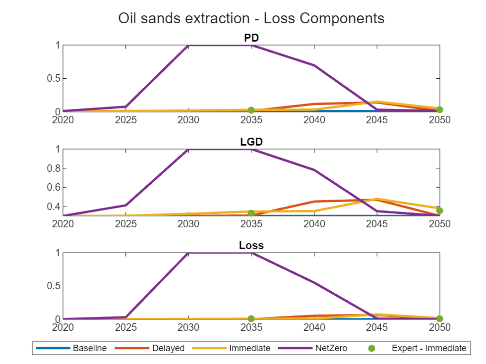
Create loss component plots at the segment level.

segmentPortfolioSummary = groupsummary(fullPortfolioPanel, ["Segment", "Year"], "mean", ... 
["ttcPD", "delayedPDPredicted", "immediatePDPredicted", "netzeroPDPredicted", ... 
"ttcLGD", "delayedLGDPredicted", "immediateLGDPredicted", "netzeroLGDPredicted", ...
"ttcLoss", "delayedLossPredicted", "immediateLossPredicted", "netzeroLossPredicted"]);

idx = ~isnan(fullPortfolioPanel.immediatePDExpert);
segmentCalibrationSummary = groupsummary(fullPortfolioPanel(idx,:), ["Segment", "Year"], "mean", ["immediatePDExpert", "immediateLGDExpert", "immediateLossExpert"]);

segment = "Oil sands extraction";
idx = segmentPortfolioSummary.Segment == segment;
segmentPortfolioData = segmentPortfolioSummary(idx, :);
idx = segmentCalibrationSummary.Segment == segment;
segmentBacktestData = segmentCalibrationSummary(idx, :);

figure;
tlo = tiledlayout(3, 1);
title(tlo, strcat(segment, " - Loss Components"));
for i = 1:numel(lossComponents)
    lossComponent = lossComponents(i);
    nexttile;
    plot(years, segmentPortfolioData.(strcat("mean_ttc", lossComponent)), 'LineWidth', 2);
    hold on;
    plot(years, segmentPortfolioData.(strcat("mean_delayed", lossComponent, "Predicted")), 'LineWidth', 2);
    plot(years, segmentPortfolioData.(strcat("mean_immediate", lossComponent, "Predicted")), 'LineWidth', 2);
    plot(years, segmentPortfolioData.(strcat("mean_netzero", lossComponent, "Predicted")), 'LineWidth', 2);
    scatter(segmentBacktestData.Year, segmentBacktestData.(strcat("mean_immediate", lossComponent, "Expert")), 'filled');
    hold off;
    title(lossComponent);
end
lg = legend("Baseline", "Delayed", "Immediate", "NetZero", "Expert - Immediate", 'Orientation', 'Horizontal', 'NumColumns', 5);
lg.Layout.Tile = 'South';

You can also use a scatter plot visualize the percent change in PD against the percent change in net income, both measured relative to the baseline at the sector level. The expectation is that net income and PD should be inversely correlated. To make this type of scatter plot, compute the change in PD relative to the baseline, then join the net income variables.

predictedPDNames = strcat(lower(scenarios), "PDPredicted");
predictedPDRelBaselineNames = strcat(predictedPDNames, "RelBaseline");
ttcPD = fullPortfolioPanel.ttcPD;

for i = 1:numel(scenarios)
    if scenarios(i) ~= "Baseline"
        predictedPDName = predictedPDNames(i);
        predictedPDRelBaselineName = predictedPDRelBaselineNames(i);
        fullPortfolioPanel.(predictedPDRelBaselineName) = (fullPortfolioPanel.(predictedPDName) - ttcPD) ./ ttcPD;
    end
end

fullPortfolioPanel = join(fullPortfolioPanel, climateDataJoin, "LeftKeys", ["Sector", "Year"], "RightKeys", ["Sector", "Year"], ...
     "RightVariables", netIncomeNames(2:end));

Next, summarize the change in PD and change in net income by sector. Then, plot the results by selecting a year and a scenario.

pdNetIncomeSector = groupsummary(fullPortfolioPanel, ["Sector", "Year"], "mean", horzcat(predictedPDRelBaselineNames(2:end), netIncomeNames(2:end)));

% Round small values to 0 for display
pdNetIncomeSectorValues = pdNetIncomeSector{:, 4:9};
pdNetIncomeSectorValues(abs(pdNetIncomeSectorValues) < threshold) = 0;
pdNetIncomeSector{:, 4:9} = pdNetIncomeSectorValues;

pdNetIncomeSector = sortrows(pdNetIncomeSector, ["Year", "Sector"]);
year = 2045;
scenario = "Delayed";
idx = pdNetIncomeSector.Year == year;

variableIdx = contains(lower(pdNetIncomeSector.Properties.VariableNames), lower(scenario + "netincome"));
netIncomeSector = 100 * pdNetIncomeSector{idx, variableIdx};

variableIdx = contains(lower(pdNetIncomeSector.Properties.VariableNames), lower(scenario + "pd"));
pdSector = 100 * pdNetIncomeSector{idx, variableIdx};

coalLabel = true;
commercialTransportationLabel = true;
cropsLabel = true;
electricityLabel = true;
energyIntensiveIndustriesLabel = true;
forestryLabel = true;
livestockLabel = true;
oilAndGasLabel = true;
refinedOilProductsLabel = true;

sectors = ["Coal", "Commercial transportation", "Crops", "Electricity", "Energy-intensive industries", "Forestry", "Livestock", "Oil & Gas", "Refined oil products"];
showSectorLabel = [coalLabel, commercialTransportationLabel, cropsLabel, electricityLabel, energyIntensiveIndustriesLabel, forestryLabel, livestockLabel, oilAndGasLabel, refinedOilProductsLabel];
sectors(~showSectorLabel) = "";

figure;
% Create offset for text labels
offset = 5;
scatter(netIncomeSector, pdSector);
xlabel("Net Income (% Change Relative to Baseline)");
ylabel("PD (% Change Relative to Baseline)");
text(netIncomeSector+offset, pdSector, sectors);
title("Year " + year + " - " + scenario);
grid on

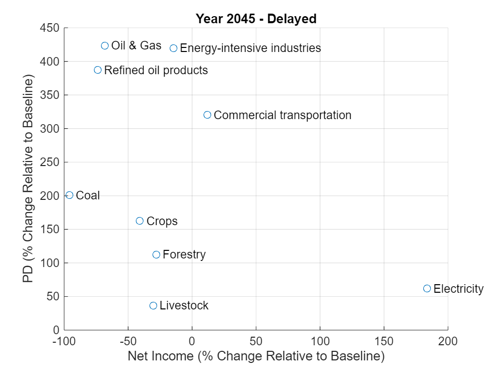
Figure contains an axes object. The axes object with title Year 2045 - Delayed, xlabel Net Income (% Change Relative to Baseline), ylabel PD (% Change Relative to Baseline) contains 10 objects of type scatter, text.

The plot shows a general negative relationship.

References

[1] UN Environment Programme Finance Initiative. Extending Our Horizons. April 2018. Available at: https://www.unepfi.org/industries/banking/extending-our-horizons/.

[2] Hosseini, H. Assessing Climate-Related Financial Risk: Guide to Implementation of Methods. Bank of Canada, 2022. Available at https://www.bankofcanada.ca/wp-content/uploads/2021/11/tr120.pdf.

[3] Office of the Superintendent of Financial Institutions. Using Scenario Analysis to Assess Climate Transition Risk. Bank of Canada, 2022. Available at https://www.bankofcanada.ca/wp-content/uploads/2021/11/BoC-OSFI-Using-Scenario-Analysis-to-Assess-Climate-Transition-Risk.pdf.

[4] UN Environment Programme Finance Initiative. Beyond the Horizon: New Tools and Frameworks for Transition Risk Assessments from UNEP FI's TCFD Banking Programme. Banking, Climate Change, Publications, Risk, TCFD. October 2020. Available at UN Environment Programme Finance Initiative.

[5] Chen, H, E. Ens, O. Gervais, H. Hosseini, C. Johnston, S. Kabaca, M. Molico, S Paltsev, A. Proulx, and A. Toktamyssov. Transition Scenarios for Analyzing Climate-Related Financial Risk. Bank of Canada, 2022. Available at https://www.bankofcanada.ca/wp-content/uploads/2021/11/sdp2022-1.pdf.

[6] Frye, Jon, and Michael Jacobs. “Credit Loss and Systematic Loss given Default.” The Journal of Credit Risk 8, no. 1 (March 2012): 109–40.

[7] https://www.bankofcanada.ca/2022/01/climate-transition-scenario-data

Assess Climate Change Impact on Credit Risk Using UNEP FI Methodology

What Is the UNEP FI Methodology?

Process Climate Scenarios and Calibration Portfolio Data

Fit the Parameters $α$ and $β$

Fit the Sensitivities

Validate the Model

Score a Portfolio

Predict LGD

Compute Losses and Aggregate Results

References

See Also

Related Topics

Assess Climate Change Impact on Credit Risk Using UNEP FI Methodology

What Is the UNEP FI Methodology?

Process Climate Scenarios and Calibration Portfolio Data

Fit the Parameters α and β

Fit the Sensitivities

Validate the Model

Score a Portfolio

Predict LGD

Compute Losses and Aggregate Results

References

See Also

Related Topics

Fit the Parameters $α$ and $β$