Credit Rating by Ordinal Multinomial Regression

Open Live Script

This example shows how to use ordinal multinomial logistic regression to build a credit rating model that you can use in an automated credit rating process.

This example assumes that historical information is available in a data set and that each record contains the features of a borrower and the assigned credit rating. These features may be internal ratings that are assigned by a committee that follow bank policies and procedures. Alternatively, the ratings may come from a rating agency that uses them to initialize a new internal credit rating system. The process of training a model on previously rated borrowers for the purpose of predicting ratings in the future is called the shadow rating or shadow bond approach.

In this example, the existing historical data is the starting point. You can use this data to train the ordinal multinomial regression model. This training process falls in the category of supervised learning. You can then use the classifier to assign ratings to new customers. In practice, these automated or predicted ratings are most likely regarded as tentative and an internal committee of credit experts reviews the automated ratings. The classifier that you use in this example facilitates revising of these credit ratings because it provides a measure of certainty for the predicted ratings, the rating probabilities.

For an introduction to credit ratings and a related modeling workflow, see Credit Rating by Bagging Decision Trees.

Load Data

Load the historical data from the comma-delimited text file CreditRating_Historical.csv. This example works with text files. If you have access to Database Toolbox™, you can load this information directly from a database.

The data set contains financial ratios, industry sectors, and credit ratings for a list of corporate borrowers. CreditRating_Historical.csv is simulated data, not real data. The first column of this data is a customer ID. The data also contains the following five columns of financial ratios:

Working Capital / Total Assets (WC_TA)
Retained Earnings / Total Assets (RE_TA)
Earnings Before Interest and Taxes / Total Assets (EBIT_TA)
Market Value of Equity / Book Value of Total Debt (MVE_BVTD)
Sales / Total Assets (S_TA)

This list of ratios are the same ratios used in Altman's Z-score (see Altman [1]; see also Loeffler and Porsch [2] for a related analysis).

The data set also includes an industry sector label. In this simulated data set, the sector is an integer value ranging from 1 to 12. In practice, the credit analyst has a mapping from the integer value to actual industry sectors. The last column has the credit rating assigned to the customer.

Load the data in a table array.

creditData = readtable("CreditRating_Historical.csv");
head(creditData)

     ID      WC_TA     RE_TA     EBIT_TA    MVE_BVTD    S_TA     Industry    Rating 
    _____    ______    ______    _______    ________    _____    ________    _______

    62394     0.013     0.104     0.036      0.447      0.142        3       {'BB' }
    48608     0.232     0.335     0.062      1.969      0.281        8       {'A'  }
    42444     0.311     0.367     0.074      1.935      0.366        1       {'A'  }
    48631     0.194     0.263     0.062      1.017      0.228        4       {'BBB'}
    43768     0.121     0.413     0.057      3.647      0.466       12       {'AAA'}
    39255    -0.117    -0.799      0.01      0.179      0.082        4       {'CCC'}
    62236     0.087     0.158     0.049      0.816      0.324        2       {'BBB'}
    39354     0.005     0.181     0.034      2.597      0.388        7       {'AA' }

Convert the industry and rating variables into categorical variables. Since the industry sectors have no natural ordering, the industry variable is nominal. On the other hand, since the credit ratings, by definition, imply a ranking of creditworthiness, the rating variable is ordinal.

creditData.Industry = categorical(creditData.Industry);

ratings = {'AAA', 'AA', 'A', 'BBB', 'BB', 'B', 'CCC'};
creditData.Rating = categorical(creditData.Rating,ratings,Ordinal=true);

Divide the data into training and test samples stratified by the credit rating.

rng(123);
partition = cvpartition(creditData.Rating, HoldOut=0.20,Stratify=true);
idTraining = training(partition);
idTest = test(partition);

creditDataTraining = creditData(idTraining, :);
creditDataTest = creditData(idTest, :);

Analyze Data

Altman's original Z-score is calculated as follows:

$Z = . 012 * W C_T A + . 014 * R E_T A + . 033 * E B I T_T A + . 006 * M V E_B V T D + . 999 * S_T A .$

According to Altman [1], a larger Z-score indicates better financial stability. As such, you expect that larger (positive) financial ratio values should be associated with better credit ratings.

Calculate the mean of each predictor variable by rating and then plot the result.

predictorVars = {'WC_TA', 'RE_TA', 'EBIT_TA', 'MVE_BVTD', 'S_TA'};
meanData = groupsummary(creditDataTraining,"Rating","mean",predictorVars);
head(meanData)

    Rating    GroupCount    mean_WC_TA    mean_RE_TA    mean_EBIT_TA    mean_MVE_BVTD    mean_S_TA
    ______    __________    __________    __________    ____________    _____________    _________

     AAA         464           0.30652      0.59523       0.075183          7.3006        0.66068 
     AA          308           0.21535      0.39472       0.062006          2.7066        0.41138 
     A           460           0.18865      0.32324        0.05898          1.8155        0.32434 
     BBB         812           0.14162       0.2172       0.053106          1.0764        0.24781 
     BB          742          0.074796     0.078795        0.04347          0.5948        0.17675 
     B           256        -0.0041484      -0.1231       0.029625         0.35907        0.14666 
     CCC         104          -0.20825     -0.91529      -0.019558         0.16476        0.11195

predictorVar = "mean_MVE_BVTD";
figure;
predictorVarTitle = extractAfter(strrep(predictorVar, '_', ' / '), 6);
bar(meanData.Rating, meanData.(predictorVar));
xlabel('Rating');
ylabel('Mean' + predictorVarTitle);
title('Mean' + predictorVarTitle + ' vs Rating');

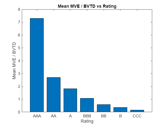
Figure contains an axes object. The axes object with title Mean MVE / BVTD vs Rating, xlabel Rating, ylabel Mean MVE / BVTD contains an object of type bar.

These plots for different predictorVar values show that each predictor has the expected monotonic relationship with the credit ratings. Thus, each predictor is a candidate for inclusion in the credit rating model.

Fit Regression Model

Based on the data analysis, you can try fitting a model with all the financial ratios included as predictors. The larger (positive) values of the predictor variables are expected to be associated with better credit ratings. In terms of the model, the coefficients of the predictor variables are expected to be positive. However, the coefficients of the predictor variables are not as expected and they have negative values.

Use fitmnr to estimate the multinomial regression model.

creditRatingModelFull = fitmnr(creditDataTraining,'Rating', ... 
    PredictorNames={'WC_TA', 'RE_TA', 'EBIT_TA', 'MVE_BVTD', 'S_TA', 'Industry'}, ...
    ModelType='ordinal')

creditRatingModelFull = 
Multinomial regression with ordinal responses

                        Value        SE        tStat       pValue   
                       ________    _______    _______    ___________

    (Intercept_AAA)      -29.83    0.90366     -33.01    5.8391e-239
    (Intercept_AA)      -22.031     0.6869    -32.073    1.0477e-225
    (Intercept_A)       -15.394    0.52426    -29.364     1.593e-189
    (Intercept_BBB)     -8.8834    0.39291     -22.61    3.4933e-113
    (Intercept_BB)      -3.5429    0.34197     -10.36     3.7611e-25
    (Intercept_B)       0.77167    0.39681     1.9447       0.051815
    WC_TA               -1.5319     1.0838    -1.4134        0.15754
    RE_TA                7.4895    0.62112     12.058     1.7584e-33
    EBIT_TA              31.849     6.9004     4.6155     3.9218e-06
    MVE_BVTD             7.6513    0.26161     29.246    4.9803e-188
    S_TA                -1.7843    0.73329    -2.4333       0.014962
    Industry_2         -0.50146    0.23203    -2.1612       0.030679
    Industry_3           2.2889    0.23437     9.7659     1.5772e-22
    Industry_4         -0.58607    0.23618    -2.4814       0.013086
    Industry_5          0.72326    0.23163     3.1224      0.0017937
    Industry_6           2.2912    0.24286     9.4344     3.9336e-21
    Industry_7           1.3539    0.23262     5.8203     5.8753e-09
    Industry_8          0.70192    0.22679      3.095      0.0019683
    Industry_9         -0.71042    0.23218    -3.0597      0.0022155
    Industry_10          -1.057    0.23019    -4.5917     4.3969e-06
    Industry_11          1.9223    0.23771     8.0867     6.1285e-16
    Industry_12         0.91313    0.23524     3.8817     0.00010375


3146 observations, 18854 error degrees of freedom
Dispersion: 1
Chi^2-statistic vs. constant model: 8332.7446, p-value = 0

Removing the variables with negative signs, $W C_T A$ and $S_T A$ , produces a model with the expected signs for all predictors. In this case, the example uses a simplified analysis and, during actual model development, a credit analyst investigates why the full model does not have the expected signs for all predictors.

The reference category CCC no intercept. One heuristic is that the reference intercept is $+ \infty$ . Therefore, the intercepts are in monotonic order, as expected.

creditRatingModel = fitmnr(creditDataTraining,'Rating', ... 
    PredictorNames={'RE_TA', 'EBIT_TA', 'MVE_BVTD', 'Industry'}, ...
    ModelType='ordinal')

creditRatingModel = 
Multinomial regression with ordinal responses

                        Value        SE        tStat       pValue   
                       ________    _______    _______    ___________

    (Intercept_AAA)      -29.75     0.8963    -33.192    1.3881e-241
    (Intercept_AA)      -22.013    0.67284    -32.717    8.9453e-235
    (Intercept_A)       -15.421    0.49656    -31.055    9.8418e-212
    (Intercept_BBB)     -8.9039    0.34906    -25.508     1.608e-143
    (Intercept_BB)      -3.5606    0.29489    -12.074      1.443e-33
    (Intercept_B)       0.70634    0.37306     1.8933       0.058311
    RE_TA                7.1973    0.59377     12.121     8.1429e-34
    EBIT_TA              26.297     4.2685     6.1607     7.2425e-10
    MVE_BVTD             7.4095    0.23391     31.676     3.336e-220
    Industry_2         -0.50867    0.23166    -2.1958       0.028109
    Industry_3           2.2767    0.23359     9.7467     1.9061e-22
    Industry_4         -0.59657    0.23586    -2.5294       0.011427
    Industry_5          0.71436    0.23083     3.0947      0.0019699
    Industry_6           2.2896    0.24274     9.4324     4.0087e-21
    Industry_7           1.3495    0.23211      5.814     6.1008e-09
    Industry_8          0.69903    0.22628     3.0893      0.0020063
    Industry_9         -0.72896    0.23189    -3.1436      0.0016688
    Industry_10         -1.0512    0.22946    -4.5812     4.6242e-06
    Industry_11          1.9104    0.23709     8.0577     7.7714e-16
    Industry_12         0.89563    0.23466     3.8166     0.00013529


3146 observations, 18856 error degrees of freedom
Dispersion: 1
Chi^2-statistic vs. constant model: 8324.8974, p-value = 0

Predict Ratings and Probabilities

You can use the multinomial regression model generated by fitmnr to predict a rating for each observation. In addition, this model provides probability estimates for each rating. The predicted rating is the favored rating. In other words, the predicted rating is equal to the rating with the highest predicted probability. Use this multinomial regression model to predict ratings on both the training data and the test data.

ratingPredictedTraining = [];
ratingPredictedTest = [];
ratingProbabilitiesTraining = [];
ratingProbabilitiesTest = [];

datasets = {creditDataTraining, creditDataTest};
for i = 1:length(datasets)
    [ratingPredicted, ratingProbabilities] = predict(creditRatingModel, datasets{i});

    ratingPredictedTable = array2table(ratingPredicted, VariableNames={'ratingPredicted'});

    ratingProbabilityNames = {'AAAProbPredicted', 'AAProbPredicted', 'AProbPredicted', 'BBBProbPredicted', 'BBProbPredicted', 'BProbPredicted', 'CCCProbPredicted'};
    ratingProbabilitiesTable = array2table(ratingProbabilities, VariableNames=ratingProbabilityNames);

    if i == 1
        ratingPredictedTraining = ratingPredictedTable;
        ratingProbabilitiesTraining = ratingProbabilitiesTable;
    else
        ratingPredictedTest = ratingPredictedTable;
        ratingProbabilitiesTest = ratingProbabilitiesTable;
    end
end

creditDataRatingsTraining = [creditDataTraining, ratingPredictedTraining, ratingProbabilitiesTraining];
creditDataRatingsTraining = addprop(creditDataRatingsTraining,PlotName="table");
creditDataRatingsTraining.Properties.CustomProperties.PlotName="Training";

creditDataRatingsTest = [creditDataTest, ratingPredictedTest, ratingProbabilitiesTest];
creditDataRatingsTest = addprop(creditDataRatingsTest,PlotName="table");
creditDataRatingsTest.Properties.CustomProperties.PlotName="Test";

Consider an individual observation from the training data. The rating with the largest predicted probability is BB. In this case, the model assigns the correct rating.

disp(creditDataRatingsTraining(1,:))

     ID      WC_TA    RE_TA    EBIT_TA    MVE_BVTD    S_TA     Industry    Rating    ratingPredicted    AAAProbPredicted    AAProbPredicted    AProbPredicted    BBBProbPredicted    BBProbPredicted    BProbPredicted    CCCProbPredicted
    _____    _____    _____    _______    ________    _____    ________    ______    _______________    ________________    _______________    ______________    ________________    _______________    ______________    ________________

    62394    0.013    0.104     0.036      0.447      0.142       3          BB            BB              1.7499e-10         4.0078e-07         0.00029215          0.16492             0.81121           0.023243          0.00033861

In this case, BB is again the rating with the largest predicted probability. However, the actual rating is BBB.

disp(creditDataRatingsTraining(5,:))

     ID      WC_TA    RE_TA    EBIT_TA    MVE_BVTD    S_TA     Industry    Rating    ratingPredicted    AAAProbPredicted    AAProbPredicted    AProbPredicted    BBBProbPredicted    BBProbPredicted    BProbPredicted    CCCProbPredicted
    _____    _____    _____    _______    ________    _____    ________    ______    _______________    ________________    _______________    ______________    ________________    _______________    ______________    ________________

    62236    0.087    0.158     0.049      0.816      0.324       2         BBB            BB              3.4514e-10         7.9046e-07         0.00057605          0.28017             0.70715           0.011925          0.00017171

Validate Regression Model

Compute the validation statistics on both the training and the test data. In general, the statistics should be comparable across these two data sets.

Since the credit ratings are ordinal, you can consider the absolute difference between the predicted and actual ratings, which are referred to as notches. All predictions are within 1 notch of the actual rating for both the training and the test data.

validationData = creditDataRatingsTraining;
notches = abs(double(validationData.Rating) - double(validationData.ratingPredicted));
figure;
histogram(notches,2,Normalization='probability');
xlabel('Notches');
ylabel('Percentage');
title(sprintf('Notch Distribution - %s', validationData.Properties.CustomProperties.PlotName));
ylim([0,1]);
xticks([0.25, 0.75]);
xticklabels({'0', '1'});

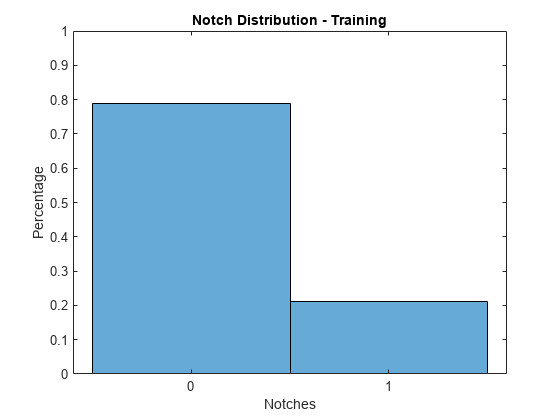
Figure contains an axes object. The axes object with title Notch Distribution - Training, xlabel Notches, ylabel Percentage contains an object of type histogram.

The accuracy rate on the training data is over 78%. The accuracy rate on the test data is higher at over 80%.

validationData = creditDataRatingsTest;

cm = confusionmat(validationData.Rating, validationData.ratingPredicted);
accuracy = sum(diag(cm)) / sum(cm(:));
fprintf('The overall accuracy on the %s data is %.2f%%\n', validationData.Properties.CustomProperties.PlotName, accuracy*100);

The overall accuracy on the Test data is 80.53%

The following confusion chart summarizes the model's predictive power. The distribution of predicted classes is similar between the training and test data, at both an overall level, and within each rating group.

figure;
cc = confusionchart(cm, ratings,ColumnSummary='total-normalized',RowSummary='total-normalized');
sortClasses(cc,ratings);
title(sprintf('Confusion Chart - %s', validationData.Properties.CustomProperties.PlotName));

Figure contains an object of type ConfusionMatrixChart. The chart of type ConfusionMatrixChart has title Confusion Chart - Test.

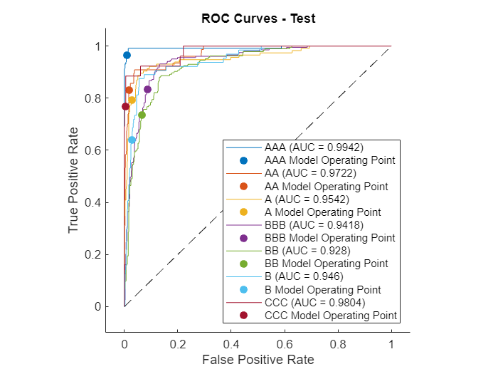
The receiver operating characteristic (ROC) curve is an additional measure of model accuracy. The ROC values are stable across all the ratings. Moreover, the values on the training and test data are comparable. Based on the ROC values, the model has strong discriminatory power.

validationData = creditDataRatingsTest;

includeRocAAA = false;
includeRocAA = true;
includeRocA = true;
includeRocBBB = true;
includeRocBB = false;
includeRocB = false;
includeRocCCC = false;
includeRoc = [includeRocAAA, includeRocAA, includeRocA, includeRocBBB, includeRocBB, includeRocB, includeRocCCC];

ratingProbabilities = validationData(:,10:16);
rocOBJ = rocmetrics(validationData.Rating, table2array(ratingProbabilities), ratings);
figure;
plot(rocOBJ, "ClassNames", ratings(includeRoc))
title(sprintf('ROC Curves - %s', validationData.Properties.CustomProperties.PlotName));

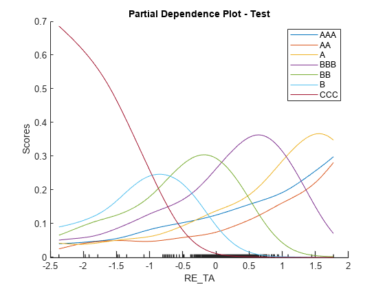
Figure contains an axes object. The axes object with title ROC Curves - Test, xlabel False Positive Rate, ylabel True Positive Rate contains 7 objects of type roccurve, scatter, line. These objects represent AA (AUC = 0.9722), AA Model Operating Point, A (AUC = 0.9542), A Model Operating Point, BBB (AUC = 0.9418), BBB Model Operating Point.

Partial dependence plots (PDPs) are an interpretability technique that allow you to examine the effect of a predictor on the overall model prediction. In this case, PDP plots help you to visualize the relationship between financial ratios and the probability of being in a particular rating class. For AAA, the curve is increasing for all variables. The relationship between each numeric predictor variable and credit quality is monotonically increasing. At the other extreme, the curves for CCC are monotonically decreasing. In other cases (for example, EBIT_TA for rating B), the curve increases, reaches a maximum, and then decreases. Once a numeric predictor increases sufficiently, it becomes more likely that the model will assign a higher rating.

validationData = creditDataRatingsTest;
includePdpAAA = true;
includePdpAA = true;
includePdpA = true;
includePdpBBB = true;
includePdpBB = true;
includePdpB = true;
includePdpCCC = true;
includePdp = [includePdpAAA, includePdpAA, includePdpA, includePdpBBB, includePdpBB, includePdpB, includePdpCCC];

figure;
plotPartialDependence(creditRatingModel,'RE_TA', ratings(includePdp), validationData)
title(sprintf('Partial Dependence Plot - %s', validationData.Properties.CustomProperties.PlotName));

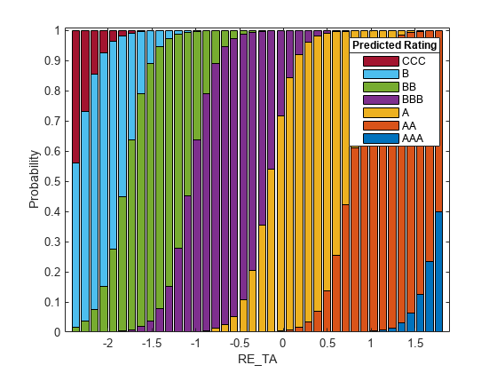
Figure contains an axes object. The axes object with title Partial Dependence Plot - Test, xlabel RE indexOf T baseline A RE_TA, ylabel Scores contains 7 objects of type line. These objects represent AAA, AA, A, BBB, BB, B, CCC.

An alternative view is to consider stacked histograms, which confirm the same trends indicated in the PDP plots.

validationData = creditDataRatingsTest;
figure;
plotSlice(creditRatingModel, "stackedhist", validationData, "PredictorToVary", "RE_TA")
lgd = legend;
title(lgd, "Predicted Rating")

Figure contains an axes object. The axes object with xlabel RE indexOf T baseline A RE_TA, ylabel Probability contains 7 objects of type bar. These objects represent AAA, AA, A, BBB, BB, B, CCC.

References

[1] Altman, E. "Financial Ratios, Discriminant Analysis and the Prediction of Corporate Bankruptcy." Journal of Finance. Vol. 23, No. 4, September 1968, pp. 589–609.

[2] Löeffler, G., and P. N. Posch. Credit Risk Modeling Using Excel and VBA. West Sussex, England, Wiley Finance, 2007.

References

[1] Baesens, B., D. Rosch, and H. Scheule. Credit Risk Analytics. Wiley, 2016, pg. 223.