Credit Rating by Bagging Decision Trees

Loading the Existing Credit Rating Data

Load the historical data from the comma-delimited text file CreditRating_Historical.dat. This example works with text files, but if you have access to Database Toolbox™, you can load this information directly from a database.

The data set contains financial ratios, industry sector, and credit ratings for a list of corporate customers. This is simulated, not real data. The first column is a customer ID. Then there are five columns of financial ratios. These are the same ratios used in Altman's z-score (see Altman [1]; see also Loeffler and Posch [4] for a related analysis).

Next, there is an industry sector label, an integer value ranging from 1 to 12. The last column has the credit rating assigned to the customer.

Load the data into a table array.

creditDS = readtable('CreditRating_Historical.dat');

Copy the features into a matrix X, and the corresponding classes, the ratings, into a vector Y. This is not a required step, since you could access this information directly from the dataset or table array, but this example does it here to simplify some repeated function calls below.

The features to be stored in the matrix X are the five financial ratios, and the industry label. Industry is a categorical variable, nominal in fact, because there is no ordering in the industry sectors. The response variable, the credit ratings, is also categorical, though this is an ordinal variable, because, by definition, ratings imply a ranking of creditworthiness. This example uses this variable "as is" to train the classifier. This variable is copied into an ordinal array because this way the outputs come out in the natural order of the ratings and are easier to read. The ordering of the ratings is established by the cell array that is passed as a third argument in the definition of Y. The credit ratings can also be mapped into numeric values, which can be useful to try alternative methods to analyze the data (for example, regression). It is always recommended to try different methods in practice.

X = [creditDS.WC_TA creditDS.RE_TA creditDS.EBIT_TA creditDS.MVE_BVTD...
     creditDS.S_TA creditDS.Industry];
Y = ordinal(creditDS.Rating);

Use the predictors X and the response Y to fit a particular type of classification ensemble called a bagged decision tree. "Bagging," in this context, stands for "bootstrap aggregation." The methodology consists in generating a number of sub-samples, or bootstrap replicas, from the data set. These sub-samples are randomly generated, sampling with replacement from the list of customers in the data set. For each replica, a decision tree is grown. Each decision tree is a trained classifier on its own, and could be used in isolation to classify new customers. The predictions of two trees grown from two different bootstrap replicas may be different, though. The ensemble aggregates the predictions of all the decision trees that are grown for all the bootstrap replicas. If the majority of the trees predict one particular class for a new customer, it is reasonable to consider that prediction to be more robust than the prediction of any single tree alone. Moreover, if a different class is predicted by a smaller set of trees, that information is useful, too. In fact, the proportion of trees that predict different classes is the basis for the classification scores that are reported by the ensemble when classifying new data.

Constructing the Tree Bagger

The first step to construct the classification ensemble will be to find a good leaf size for the individual trees; here the example tries sizes of 1, 5, and 10. (See Statistics and Machine Learning Toolbox documentation for more on TreeBagger.) Start with a small number of trees, 25 only, because you mostly want to compare the initial trend in the classification error for different leaf sizes. For reproducibility and fair comparisons, reinitialize the random number generator, which is used to sample with replacement from the data, each time you build a classifier.

leaf = [1 5 10];
nTrees = 25;
rng(9876,'twister');
savedRng = rng; % Save the current RNG settings

color = 'bgr';
for ii = 1:length(leaf)
   % Reinitialize the random number generator, so that the
   % random samples are the same for each leaf size
   rng(savedRng)
   % Create a bagged decision tree for each leaf size and plot out-of-bag
   % error 'oobError'
   b = TreeBagger(nTrees,X,Y,'OOBPrediction','on',...
                             'CategoricalPredictors',6,...
                             'MinLeafSize',leaf(ii));
   plot(oobError(b),color(ii))
   hold on
end
xlabel('Number of grown trees')
ylabel('Out-of-bag classification error')
legend({'1', '5', '10'},'Location','NorthEast')
title('Classification Error for Different Leaf Sizes')
hold off

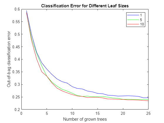
The errors are comparable for the three leaf-size options. Therefore work with a leaf size of 10, because it results in leaner trees and more efficient computations.

Note that you did not have to split the data into training and test subsets. This is done internally, it is implicit in the sampling procedure that underlies the method. At each bootstrap iteration, the bootstrap replica is the training set, and any customers left out ("out-of-bag") are used as test points to estimate the out-of-bag classification error reported above.

Next, find out whether all the features are important for the accuracy of the classifier. Do this by turning on the feature importance measure (OOBPredictorImportance), and plot the results to visually find the most important features. Now try a larger number of trees and store the classification error, for further comparisons below.

nTrees = 50;
leaf = 10;
rng(savedRng);
b = TreeBagger(nTrees,X,Y,'OOBPredictorImportance','on', ...
                          'CategoricalPredictors',6, ...
                          'MinLeafSize',leaf);

bar(b.OOBPermutedPredictorDeltaError)
xlabel('Feature number')
ylabel('Out-of-bag feature importance')
title('Feature importance results')

oobErrorFullX = oobError(b);

Features 2, 4 and 6 stand out from the rest. Feature 4, market value of equity / book value of total debt (MVE_BVTD), is the most important predictor for this data set. This ratio is closely related to the predictors of creditworthiness in structural models, such as Merton's model [5], where the value of the firm's equity is compared to its outstanding debt to determine the default probability.

Information on the industry sector, feature 6 (Industry), is also relatively more important than other variables to assess the creditworthiness of a firm for this data set.

Although not as important as MVE_BVTD, feature 2, retained earnings / total assets (RE_TA), stands out from the rest. There is a correlation between retained earnings and the age of a firm (the longer a firm has existed, the more earnings it can accumulate, in general), and in turn the age of a firm is correlated to its creditworthiness (older firms tend to be more likely to survive in tough times).

Fit a new classification ensemble using only predictors RE_TA, MVE_BVTD, and Industry. Compare its classification error with the previous classifier, which uses all features.

X = [creditDS.RE_TA creditDS.MVE_BVTD creditDS.Industry];

rng(savedRng)
b = TreeBagger(nTrees,X,Y,'OOBPrediction','on', ...
                          'CategoricalPredictors',3, ...
                          'MinLeafSize',leaf);

oobErrorX246 = oobError(b);

plot(oobErrorFullX,'b')
hold on
plot(oobErrorX246,'r')
xlabel('Number of grown trees')
ylabel('Out-of-bag classification error')
legend({'All features', 'Features 2, 4, 6'},'Location','NorthEast')
title('Classification Error for Different Sets of Predictors')
hold off

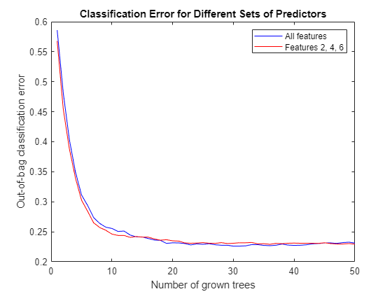
The accuracy of the classification does not deteriorate significantly when you remove the features with relatively low importance (1, 3, and 5), so you will use the more parsimonious classification ensemble for the predictions.

This example started with a set of only six features, and used the feature importance measure of the classifier, and the out-of-bag classification error as criteria to screen out three of the variables. Feature selection can be a time consuming process when the initial set of potential predictors contains dozens of variables. Besides the tools used here (variable importance and a "visual" comparison of out-of-bag errors), other variable selection tools in Statistics and Machine Learning Toolbox can be helpful for these types of analyses. However, in the end, a successful feature selection process requires a combination of quantitative tools and an analyst's judgement.

For example, the variable importance measure used here is a ranking mechanism that estimates the relative impact of a feature by measuring how much the predictive accuracy of the classifier deteriorates when this feature's values are randomly permuted. The idea is that when the feature in question adds little to the predictive power of the classifier, using altered (in this case permuted) values should not impact the classification results. Relevant information, on the other hand, cannot be randomly swapped without degrading the predictions. Now, if two highly correlated features are important, they will both rank high in this analysis. In that case, keeping one of these features should suffice for accurate classifications, but you would not know that from the ranking results alone. You would have to check the correlations separately, or use an expert's judgement. That is to say, tools like variable importance or sequentialfs can greatly help for feature selection, but an analyst's judgment is a key piece in this process.

At this point, the classifier could be saved (for example, save classifier.mat b), to be loaded in a future session (load classifier) to classify new customers. For efficiency, it is recommended to keep a compact version of the classifier once the training process is finished.

b = compact(b);

Classifying New Data

Use the previously constructed classification ensemble to assign credit ratings to new customers. Because the ratings of existing customers need to be reviewed, too, on a regular basis, especially when their financial information has substantially changed, the data set could also contain a list of existing customers under review. Start by loading the new data.

newDS = readtable('CreditRating_NewCompanies.dat');

To predict the credit rating for this new data, call the predict method on the classifier. The method returns two arguments, the predicted class and the classification score. You certainly want to get both output arguments, since the classification scores contain information on how certain the predicted ratings seem to be. You could copy variables RE_TA, MVE_BVTD and Industry into a matrix X, as before, but since you will make only one call to predict, you can skip this step and use newDS directly.

[predClass,classifScore] = predict(b,[newDS.RE_TA newDS.MVE_BVTD newDS.Industry]);

At this point, you can create a report. Here this example only displays on the screen a small report for the first three customers, for illustration purposes, but MATLAB deployment tools could greatly improve the workflow here. For example, credit analysts could run this classification remotely, using a web browser, and get a report, without even having MATLAB on their desktops.

for i = 1:3
   fprintf('Customer %d:\n',newDS.ID(i));
   fprintf('   RE/TA    = %5.2f\n',newDS.RE_TA(i));
   fprintf('   MVE/BVTD = %5.2f\n',newDS.MVE_BVTD(i));
   fprintf('   Industry = %2d\n',newDS.Industry(i));
   fprintf('   Predicted Rating : %s\n',predClass{i});
   fprintf('   Classification score : \n');
   for j = 1:length(b.ClassNames)
      if (classifScore(i,j)>0)
         fprintf('      %s : %5.4f \n',b.ClassNames{j},classifScore(i,j));
      end
   end
end

Customer 60644:

   RE/TA    =  0.22

   MVE/BVTD =  2.40

   Industry =  6

   Predicted Rating : AA

   Classification score : 

      A : 0.2349 
      AA : 0.7519 
      AAA : 0.0011 
      BBB : 0.0121 

Customer 33083:

   RE/TA    =  0.24

   MVE/BVTD =  1.51

   Industry =  4

   Predicted Rating : BBB

   Classification score : 

      A : 0.1060 
      BBB : 0.8940 

Customer 63830:

   RE/TA    =  0.18

   MVE/BVTD =  1.69

   Industry =  7

   Predicted Rating : A

   Classification score : 

      A : 0.6305 
      AA : 0.0172 
      AAA : 0.0010 
      BBB : 0.3513 

Keeping records of the predicted ratings and corresponding scores can be useful for periodic assessments of the quality of the classifier. You can store this information in the table array predDS.

classnames = b.ClassNames;
predDS = [table(newDS.ID,predClass),array2table(classifScore)];
predDS.Properties.VariableNames = [{'ID'},{'PredRating'},classnames'];

This information could be saved, for example, to a comma-delimited text file PredictedRatings.dat using the command

  writetable(predDS,'PredictedRatings.dat');

or written directly to a database using Database Toolbox.

Back-Testing: Profiling the Classification Process

Validation or back-testing is the process of profiling or assessing the quality of the credit ratings. There are many different measures and tests related to this task (see, for example, Basel Committee on Banking Supervision [2]). Here, this example focuses on the following two questions:

The file CreditRating_ExPost.dat contains "follow up" data on the same companies considered in the previous section. It contains the actual ratings that the committee assigned to these companies, as well as a "default flag" that indicates whether the corresponding company defaulted within one year of the rating process (if 1) or not (if 0).

exPostDS = readtable('CreditRating_ExPost.dat');

Comparing predicted ratings vs. actual ratings.

The rationale to train an automated classifier is to expedite the work of the credit committee. The more accurate the predicted ratings are, the less time the committee has to spend reviewing the predicted ratings. So it is conceivable that the committee wants to have regular checks on how closely the predicted ratings match the final ratings they assign, and to recommend re-training the automated classifier (and maybe include new features, for example) if the mismatch seems concerning.

The first tool you can use to compare predicted vs. actual ratings is a confusion matrix, readily available in Statistics and Machine Learning Toolbox:

C = confusionchart(exPostDS.Rating,predDS.PredRating);
sortClasses(C,{'AAA' 'AA' 'A' 'BBB' 'BB' 'B' 'CCC'})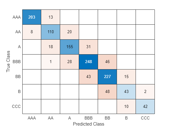

The rows correspond to the actual ratings, and the columns to the predicted ratings. The amount in the position (i,j) in the confusion matrix indicates how many customers received an actual rating i and were predicted as rating j. For example, position (3,2) tells us how many customers received a rating of 'A' by the credit committee, but were predicted as 'AA' with the automated classifier. You can also present this matrix in percentage. Normalize each value by the number of observations that has the same true rating.

C.Normalization = 'row-normalized';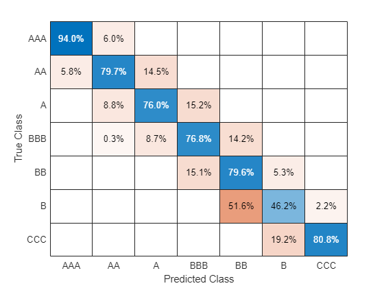

Good agreement between the predicted and the actual ratings would result in values in the main diagonal that dominate the rest of the values in a row, ideally values close to 1. In this case, you can actually see an important disagreement for 'B', since about half of the customers that were rated as 'B' by the credit committee had been predicted as 'BB' by the automated classifier. On the other hand, it is good to see that ratings differ in at most one notch in most cases, with the only exception of 'BBB'.

A confusion matrix could also be used to compare the internal ratings assigned by the institution against third-party ratings; this is often done in practice.

For each specific rating, you can compute another measure of agreement between predicted and actual ratings. You can build a Receiver Operating Characteristic (ROC) curve and check the area under the curve (AUC) by using the rocmetrics object. rocmetrics takes the actual ratings (the standard you are comparing against) and the 'BBB' classification scores determined by the automated process.

rocObj1 = rocmetrics(exPostDS.Rating,predDS.BBB,'BBB');

Plot the ROC curve for the rating 'BBB' by using the plot function of rocmetrics.

plot(rocObj1)

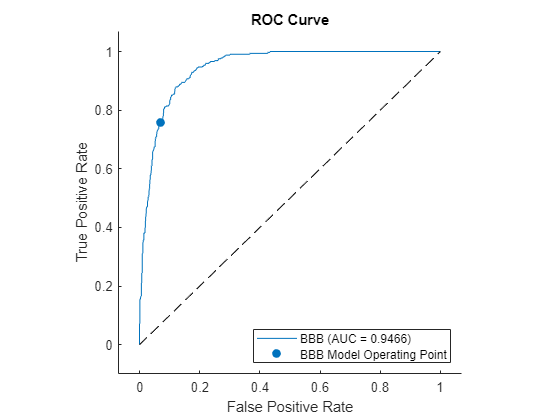
Here is an explanation of how the ROC is built. Recall that for each customer the automated classifier returns a classification score for each of the credit ratings, in particular, for 'BBB', which can be interpreted as how likely it is that this particular customer should be rated 'BBB'. In order to build the ROC curve, you need to vary the classification threshold. That is, the minimum score to classify a customer as 'BBB'. In other words, if the threshold is t, you only classify customers as 'BBB' if their 'BBB' score is greater than or equal to t. For example, suppose that company XYZ had a 'BBB' score of 0.87. If the actual rating of XYZ (the information in exPostDS.Rating) is 'BBB', then XYZ would be correctly classified as 'BBB' for any threshold of up to 0.87. This would be a true positive, and it would increase what is called the sensitivity of the classifier. For any threshold greater than 0.87, this company would not receive a 'BBB' rating, and you would have a false negative case. To complete the description, suppose now that XYZ's actual rating is 'BB'. Then it would be correctly rejected as a 'BBB' for thresholds of more than 0.87, becoming a true negative, and thus increasing the so called specificity of the classifier. However, for thresholds of up to 0.87, it would become a false positive (it would be classified as 'BBB', when it actually is a 'BB'). The ROC curve is constructed by plotting the proportion of true positives (sensitivity), versus false positives (1-specificity), as the threshold varies from 0 to 1.

The AUC, as its name indicates, is the area under the ROC curve. The closer the AUC is to 1, the more accurate the classifier (a perfect classifier would have an AUC of 1). In this example, the AUC seems high enough, but it would be up to the committee to decide which level of AUC for the ratings should trigger a recommendation to improve the automated classifier.

Comparing actual ratings vs. defaults in the following year.

A common tool used to assess the ranking of customers implicit in the credit ratings is the Cumulative Accuracy Profile (CAP), and the associated accuracy ratio measure. The idea is to measure the relationship between the credit ratings assigned and the number of defaults observed in the following year. One would expect that fewer defaults are observed for better rating classes. If the default rate were the same for all ratings, the rating system would be no different from a naive (and useless) classification system in which customers were randomly assigned a rating, independently of their creditworthiness.

It is not hard to see that rocmetrics can also be used to construct the CAP. The standard compared against is not a rating, as before, but the default flag that is loaded from the CreditRating_ExPost.dat file. The score that you use is a "dummy score" that indicates the ranking in creditworthiness implicit in the list of ratings. The dummy score only needs to satisfy that better ratings get lower dummy scores (they are "less likely to have a default flag of 1"), and that any two customers with the same rating get the same dummy score. A default probability could be passed as a score, of course, but you do not have default probabilities here, and in fact you do not need to have estimates of the default probabilities to construct the CAP, because you are not validating default probabilities. All that this example is assessing with this tool is how well the ratings rank customers according to their creditworthiness.

Usually, the CAP of the rating system under consideration is plotted together with the CAP of the "perfect rating system." The latter is a hypothetical credit rating system for which the lowest rating includes all the defaulters, and no other customers. The area under this perfect curve is the maximum possible AUC attainable by a rating system. By convention, the AUC is adjusted for CAPs to subtract the area under the naive system's CAP, that is, the CAP of the system that randomly assigns ratings to customers. The naive system's CAP is simply a straight line from the origin to (1,1), with an AUC of 0.5. The accuracy ratio for a rating system is then defined as the ratio of the adjusted AUC (AUC of the system in consideration minus AUC of the naive system) to the maximum accuracy (AUC of the perfect system minus AUC of the naive system).

ratingsList = {'AAA' 'AA' 'A' 'BBB' 'BB' 'B' 'CCC'};
Nratings = length(ratingsList);
dummyDelta = 1/(Nratings+1);
dummyRank = linspace(dummyDelta,1-dummyDelta,Nratings)';

D = exPostDS.Def_tplus1;
fracTotDef = sum(D)/length(D);
maxAcc = 0.5 - 0.5 * fracTotDef;

R = double(ordinal(exPostDS.Rating,[],ratingsList));
S = dummyRank(R);
rocObj2 = rocmetrics(D,S,1);
xVal = rocObj2.Metrics.FalsePositiveRate;
yVal = rocObj2.Metrics.TruePositiveRate;
auc = rocObj2.AUC;

accRatio = (auc-0.5)/maxAcc;
fprintf('Accuracy ratio for actual ratings: %5.3f\n',accRatio);

Accuracy ratio for actual ratings: 0.850

xPerfect(1) = 0; xPerfect(2) = fracTotDef; xPerfect(3) = 1;
yPerfect(1) = 0; yPerfect(2) = 1; yPerfect(3) = 1;
xNaive(1) = 0; xNaive(2) = 1;
yNaive(1) = 0; yNaive(2) = 1;

plot(xPerfect,yPerfect,'--k',xVal,yVal,'b',xNaive,yNaive,'-.k')
xlabel('Fraction of all companies')
ylabel('Fraction of defaulted companies')
title('Cumulative Accuracy Profile')
legend({'Perfect','Actual','Naive'},'Location','SouthEast')
text(xVal(2)+0.01,yVal(2)-0.01,'CCC')
text(xVal(3)+0.01,yVal(3)-0.02,'B')
text(xVal(4)+0.01,yVal(4)-0.03,'BB')

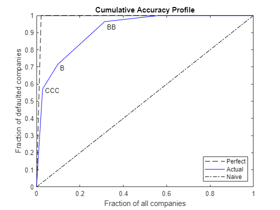
The key to reading the information of the CAP is in the "kinks," labeled in the plot for ratings 'CCC', 'B', and 'BB'. For example, the second kink is associated with the second lowest rating, 'B', and it is located at (0.097, 0.714). This means that 9.7% of the customers were ranked 'B' or lower, and they account for 71.4% of the defaults observed.

In general, the accuracy ratio should be treated as a relative, rather than an absolute measure. For example, you can add the CAP of the predicted ratings in the same plot, and compute its accuracy ratio to compare it with the accuracy ratio of the actual ratings.

Rpred = double(ordinal(predDS.PredRating,[],ratingsList));
Spred = dummyRank(Rpred);
rocObj3 = rocmetrics(D,Spred,1);
xValPred = rocObj3.Metrics.FalsePositiveRate;
yValPred = rocObj3.Metrics.TruePositiveRate;
aucPred = rocObj3.AUC;

accRatioPred = (aucPred-0.5)/maxAcc;
fprintf('Accuracy ratio for predicted ratings: %5.3f\n',accRatioPred);

Accuracy ratio for predicted ratings: 0.811

plot(xPerfect,yPerfect,'--k',xVal,yVal,'b',xNaive,yNaive,'-.k',...
   xValPred,yValPred,':r')
xlabel('Fraction of all companies')
ylabel('Fraction of defaulted companies')
title('Cumulative Accuracy Profile')
legend({'Perfect','Actual','Naive','Predicted'},'Location','SouthEast')

The accuracy ratio of the predicted rating is smaller, and its CAP is mostly below the CAP of the actual rating. This is reasonable, since the actual ratings are assigned by the credit committees that take into consideration the predicted ratings and extra information that can be important to fine-tune the ratings.

Final Remarks

MATLAB offers a wide range of machine learning tools, besides bagged decision trees, that can be used in the context of credit rating. In Statistics and Machine Learning Toolbox you can find classification tools such as discriminant analysis and naive Bayes classifiers. MATLAB also offers Deep Learning Toolbox™. Also, Database Toolbox and MATLAB deployment tools may provide you with more flexibility to adapt the workflow presented here to your own preferences and needs.

No probabilities of default have been computed here. For credit ratings, the probabilities of default are usually computed based on credit-rating migration history. See the transprob (Financial Toolbox) reference page in Financial Toolbox™ for more information.

Bibliography

[1] Altman, E. "Financial Ratios, Discriminant Analysis and the Prediction of Corporate Bankruptcy." Journal of Finance. Vol. 23, No. 4, (September 1968), pp. 589-609.

[2] Basel Committee on Banking Supervision. "Studies on the Validation of Internal Rating Systems." Bank for International Settlements (BIS), Working Papers No. 14, revised version, May 2005. Available at: https://www.bis.org/publ/bcbs_wp14.htm.

[3] Basel Committee on Banking Supervision. "International Convergence of Capital Measurement and Capital Standards: A Revised Framework." Bank for International Settlements (BIS), comprehensive version, June 2006. Available at: https://www.bis.org/publ/bcbsca.htm.

[4] Loeffler, G., and P. N. Posch. Credit Risk Modeling Using Excel and VBA. West Sussex, England: Wiley Finance, 2007.

[5] Merton, R. "On the Pricing of Corporate Debt: The Risk Structure of Interest Rates." Journal of Finance. Vol. 29, No. 2, (May, 1974), pp. 449-70.