Estimate Portfolio-Level LGD with Frye-Jacobs Function

Open Live Script

The fryeJacobsLGD function allows you to predict the conditional loss given default (LGD) as a function of the conditional probability of default (PD). You can use this function to incorporate LGD risk into your modeling scenarios by using it to estimate the portfolio-level LGD for various PD levels. In this example, you use the function to estimate the LGD during a year in which a portfolio experiences a stressed default rate.

Estimate Input Arguments

First, load the data, which represents the annual default rate and LGD rate for a portfolio of bank exposures.

load("AnnualCreditPortfolioData.mat")
disp(annualPortfolioData)

    Year    DefaultRate    LGDRate
    ____    ___________    _______

    2010       0.048       0.58277
    2011        0.02        0.5368
    2012        0.01       0.51874
    2013       0.038       0.52944
    2014       0.039       0.63319
    2015       0.012       0.45097
    2016        0.05       0.61295
    2017       0.044       0.56352
    2018       0.018       0.47346
    2019       0.015       0.53689

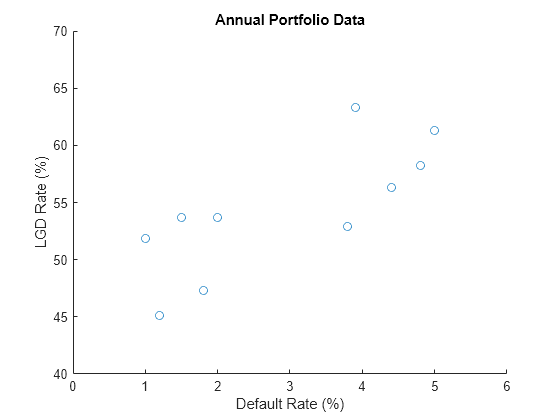
Visualize the portfolio data by making a scatter plot of the default rate and the LGD rate.

figure;
scatter(100*annualPortfolioData.DefaultRate,100*annualPortfolioData.LGDRate);
xlabel("Default Rate (%)");
xlim([0,6]);
ylabel("LGD Rate (%)");
ylim([40,70]);
title("Annual Portfolio Data");

Figure contains an axes object. The axes object with title Annual Portfolio Data, xlabel Default Rate (%), ylabel LGD Rate (%) contains an object of type scatter.

The fryeJacobsLGD function requires you to specify four required input arguments that include: ConditionalPD, BaselinePD, BaselineLGD, and Correlation.

ConditionalPD is sometimes called the conditional default rate in the financial literature. In stress testing applications, this might be a stressed or forecasted PD.
BaselinePD is sometimes called the probability of default in the financial literature. It is often regarded as a through-the-cycle or a priori PD.
BaselineLGD is sometimes called the expected LGD. It is often regarded as a through-the-cycle or a priori LGD.
Correlation is often regarded as $ρ$ in the financial literature. For information on estimating Correlation, see Calculating Regulatory Capital with the ASRF Model.

Before you use the fryeJacobsLGD function, you need to estimate the BaselinePD, the BaselineLGD, and the Correlation input arguments.

For the BaselinePD estimate, use the average annual default rate:

BaselinePDEstimate = mean(annualPortfolioData.DefaultRate);
disp(BaselinePDEstimate)

    0.0294

You can estimate the BaselineLGD by calculating the average annual LGD rate:

BaselineLGDAverage = mean(annualPortfolioData.LGDRate);
disp(BaselineLGDAverage)

    0.5439

Alternatively, you can calculate the average annual loss rate using the relation Loss Rate = Defalut Rate*LGD Rate:

lossRate = annualPortfolioData.DefaultRate.*annualPortfolioData.LGDRate;
disp(lossRate)

averageAnnualLossRate = mean(lossRate);
disp(averageAnnualLossRate)

    0.0166

BaselineLGDWeighted = averageAnnualLossRate/BaselinePDEstimate;
disp(BaselineLGDWeighted)

    0.5651

Note that this estimate is slightly higher than the first estimate, which reflects the fact that LGD tends to increase with default rate.

Finally, estimate the correlation by using the Basel formula as follows:

CorrelationEstimate = 0.12*(1-exp(-50*BaselinePDEstimate))/(1-exp(-50)) + ...
    0.24*(1-(1-exp(-50*BaselinePDEstimate))/(1-exp(-50)));
disp(CorrelationEstimate)

    0.1476

For details on using this formula, see Calculating Regulatory Capital with the ASRF Model. In addition to the Basel estimate, you can consider the values 0.12 and 0.24 for the correlation, which represent the extreme values according to the Basel formula.

CorrelationMin = 0.12;
CorrelationMax = 0.24;

Effects of BaselineLGD and Correlation on LGD

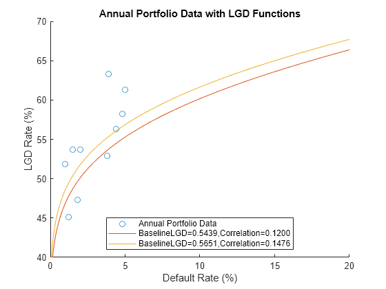
Visualize how the BaselineLGD and Correlation affect the conditional LGD by considering all combinations of their estimates which results in a total of six LGD functions. Compare two at a time to see how changes to the BaselineLGD and Correlation estimates affect the LGD function:

BaselineLGD1 = BaselineLGDAverage;
BaselineLGD2 = BaselineLGDWeighted;
Correlation1 = CorrelationMin;
Correlation2 = CorrelationEstimate;

figure;
scatter(100*annualPortfolioData.DefaultRate,100*annualPortfolioData.LGDRate,"DisplayName","Annual Portfolio Data");
xlabel("Default Rate (%)");
xlim([0,20]);
ylabel("LGD Rate (%)");
ylim([40,70]);
title("Annual Portfolio Data with LGD Functions");
hold on;
ConditionalPD = linspace(1e-10,0.2,1000)';
ConditionalLGD1 = fryeJacobsLGD(ConditionalPD,BaselinePDEstimate,BaselineLGD1,Correlation1);
plot(100*ConditionalPD,100*ConditionalLGD1,"DisplayName",sprintf("BaselineLGD=%.4f,Correlation=%.4f",BaselineLGD1,Correlation1));
ConditionalLGD2 = fryeJacobsLGD(ConditionalPD,BaselinePDEstimate,BaselineLGD2,Correlation2);
plot(100*ConditionalPD,100*ConditionalLGD2,"DisplayName",sprintf("BaselineLGD=%.4f,Correlation=%.4f",BaselineLGD2,Correlation2));
legend("Location","best");
hold off;

Figure contains an axes object. The axes object with title Annual Portfolio Data with LGD Functions, xlabel Default Rate (%), ylabel LGD Rate (%) contains 3 objects of type scatter, line. These objects represent Annual Portfolio Data, BaselineLGD=0.5439,Correlation=0.1200, BaselineLGD=0.5651,Correlation=0.1476.

These functions provide reasonable estimates for the LGD rate for different levels of observed default rates or conditional PD rates. For this portfolio, the largest annual default rate was 5% in 2016.

Estimate LGD with Stressed Default Rate

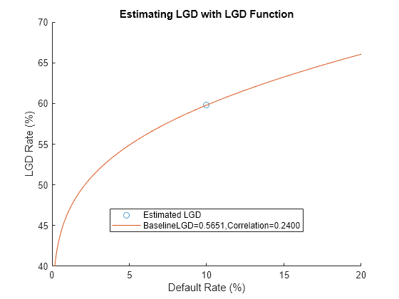
Use the fryeJacobsLGD function to estimate the conditional LGD with a stressed default rate. In this example, assume the default rate next year is 10% and estimate the LGD. Choose combinations of the BaselineLGD and Correlation input arguments and visualize their effect on the LGD Rate.

ConditionalPD = 0.10;
BaselineLGD = BaselineLGDWeighted;
Correlation = CorrelationMax;
estimatedLGD = fryeJacobsLGD(ConditionalPD,BaselinePDEstimate,BaselineLGD,Correlation);
disp(estimatedLGD)

    0.5980

figure;
scatter(100*ConditionalPD,100*estimatedLGD,"DisplayName","Estimated LGD");
xlabel("Default Rate (%)");
xlim([0,20]);
ylabel("LGD Rate (%)");
ylim([40,70]);
title("Estimating LGD with LGD Function");
hold on;
ConditionalPD = linspace(1e-10,0.2,1000)';
ConditionalLGD = fryeJacobsLGD(ConditionalPD,BaselinePDEstimate,BaselineLGD,Correlation);
plot(100*ConditionalPD,100*ConditionalLGD,"DisplayName",sprintf("BaselineLGD=%.4f,Correlation=%.4f",BaselineLGD,Correlation));
legend("Location","best");
hold off;

Figure contains an axes object. The axes object with title Estimating LGD with LGD Function, xlabel Default Rate (%), ylabel LGD Rate (%) contains 2 objects of type scatter, line. These objects represent Estimated LGD, BaselineLGD=0.5651,Correlation=0.2400.

References

[1] Frye, Jon, and Michael Jacobs. “Credit Loss and Systematic Loss given Default.” The Journal of Credit Risk 8, no. 1 (March 2012): 109–40.

[2] Frye, Jon. “The simple link from default to LGD.” Risk, London (March 2014): 60–65.

Estimate Portfolio-Level LGD with Frye-Jacobs Function

Estimate Input Arguments

Effects of BaselineLGD and Correlation on LGD

Estimate LGD with Stressed Default Rate

References

See Also

Related Topics