Mobile Robot Kinematics Equations

Open Live Script

Learn details about mobile robot kinematics equations including unicycle, bicycle, differential drive, and Ackermann models. This topic covers the variables and specific equations for each motion model [1]. For an example that simulates the different mobile robots using these models, see Simulate Different Kinematic Models for Mobile Robots.

Variable Overview

The robot state is represented as a three-element vector: [ $x$ $y$ $θ$ ].

For a given robot state:

$x$ : Global vehicle x-position in meters
$y$ : Global vehicle y-position in meters
$θ$ : Global vehicle heading in radians

For Ackermann kinematics, the state also includes steering angle:

$ψ$ : Vehicle steering angle in radians

The unicycle, bicycle, and differential drive models share a generalized control input, which accepts the following:

$v$ : Vehicle speed in meters/s
$ω$ : Vehicle angular velocity in radians/s

Other variables represented in the kinematics equations are:

$r$ : Wheel radius in meters
$ϕ_{}^{˙}$ : Wheel speed in radians/s
$d$ : Track width in meters
$l$ : Wheel base in meters
$ψ$ : Vehicle steering angle in radians

Unicycle Kinematics

The unicycle kinematics equations model a single rolling wheel that pivots about a central axis using the unicycleKinematics object.

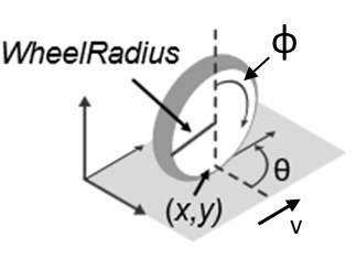
The unicycle model state is [ $x$ $y$ $θ$ ].

Variables

$x$ : Global vehicle x-position in meters
$y$ : Global vehicle y-position in meters
$θ$ : Global vehicle heading in radians
$ϕ_{}^{˙}$ : Wheel speed in meters/s
$r$ : Wheel radius in meters
$v$ : Vehicle speed in meters/s
$ω$ : Vehicle heading angular velocity in radians/s

Kinematic Equations

Depending on the VehicleInputs name-value argument, you can input only wheel speeds or the vehicle speed and heading rate. This change in input affects the equations.

Wheel Speed Equation

$[\begin{array}{cc} x_{}^{˙} \\ y_{}^{˙} \\ θ_{}^{˙} \end{array}] = [\begin{array}{cc} r \cos (θ) & 0 \\ r \sin (θ) & 0 \\ 0 & 1 \end{array}] [\begin{array}{cc} ϕ_{}^{˙} \\ ω \end{array}]$

Vehicle Speed and Heading Rate Equation (Generalized)

When the generalized inputs are given as the speed $v = r ϕ_{}^{˙}$ and vehicle heading angular velocity $ω$ , the equation simplifies to:

$[\begin{array}{cc} x_{}^{˙} \\ y_{}^{˙} \\ θ_{}^{˙} \end{array}] = [\begin{array}{cc} \cos (θ) & 0 \\ \sin (θ) & 0 \\ 0 & 1 \end{array}] [\begin{array}{cc} v \\ ω \end{array}]$

Bicycle Kinematics

The bicycle kinematics equations model a car-like vehicle that accepts the front steering angle as a control input using the bicycleKinematics object.

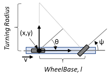
The bicycle model state is [ $x$ $y$ $θ$ ].

Variables

$x$ : Global vehicle x-position in meters
$y$ : Global vehicle y-position in meters
$θ$ : Global vehicle heading in radians
$l$ : Wheel base, in meters
$ψ$ : Vehicle steering angle in radians
$v$ : Vehicle speed in meters/s
$ω$ : Vehicle heading angular velocity in radians/s

Kinematic Equations

Depending on the VehicleInputs name-value argument, you can input the vehicle speed as either the steering angle or heading rate. This change in input affects the equations.

Steering Angle Equation

$[\begin{array}{cc} x_{}^{˙} \\ y_{}^{˙} \\ θ_{}^{˙} \end{array}] = [\begin{array}{cc} c o s (θ) & 0 \\ s i n (θ) & 0 \\ \frac{\tan (ψ)}{l} & 1 \end{array}] [\begin{array}{cc} v \\ ω \end{array}]$

Vehicle Speed and Heading Rate Equation (Generalized)

In this generalized format, the heading rate $ω$ can be related to the steering angle $ψ$ with the relation $ω = \frac{v}{l} \tan ψ$ . Then, the ODE simplifies to:

$[\begin{array}{cc} x_{}^{˙} \\ y_{}^{˙} \\ θ_{}^{˙} \end{array}] = [\begin{array}{cc} \cos (θ) & 0 \\ \sin (θ) & 0 \\ 0 & 1 \end{array}] [\begin{array}{cc} v \\ ω \end{array}]$

Differential Drive Kinematics

The differential drive kinematics equations model a vehicle where the wheels on the left and right may spin independently using the differentialDriveKinematics object.

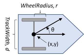
The differential drive model state is [ $x$ $y$ $θ$ ].

Variables

$x$ : Global vehicle x-position, in meters
$y$ : Global vehicle y-position, in meters
$θ$ : Global vehicle heading, in radians
${ϕ_{}^{˙}}_{L}$ : Left wheel speed in meters/s
${ϕ_{}^{˙}}_{R}$ : Right wheel speed in meters/s
$r$ : Wheel radius in meters
$d$ : Track width in meters
$v$ : Vehicle speed in meters/s
$ω$ : Vehicle heading angular velocity in radians/s

Kinematic Equations

Depending on the VehicleInputs name-value argument, you can input the wheel speed as either the steering angle or heading rate. This change in input affects the equations.

Wheel Speed Equation

$[\begin{array}{cc} x_{}^{˙} \\ y_{}^{˙} \\ θ_{}^{˙} \end{array}] = [\begin{array}{cc} \frac{r}{2} \cos (θ) & \frac{r}{2} \cos (θ) \\ \frac{r}{2} \sin (θ) & \frac{r}{2} \sin (θ) \\ - r / d & r / d \end{array}] [\begin{array}{cc} {ϕ_{}^{˙}}_{L} \\ {ϕ_{}^{˙}}_{R} \end{array}]$

Vehicle Speed and Heading Rate Equation (Generalized)

In the generalized format, the inputs are given as the speed $v = \frac{r}{2} ({ϕ_{}^{˙}}_{R} + {ϕ_{}^{˙}}_{L})$ and vehicle heading angular velocity $ω = \frac{r}{d} ({ϕ_{}^{˙}}_{R} - {ϕ_{}^{˙}}_{L})$ . The ODE simplifies to:

$[\begin{array}{cc} x_{}^{˙} \\ y_{}^{˙} \\ θ_{}^{˙} \end{array}] = [\begin{array}{cc} \cos (θ) & 0 \\ \sin (θ) & 0 \\ 0 & 1 \end{array}] [\begin{array}{cc} v \\ ω \end{array}]$

Ackermann Kinematics

The Ackermann kinematic equations model a car-like vehicle model with an Ackermann-steering mechanism using the ackermannKinematics object. The equation adjusts the position of the axle tires based on the track width so that the tires follow concentric circles. Mathematically, this means that the input has to be the steering heading angular velocity $ψ_{}^{˙}$ , and there is no generalized format.

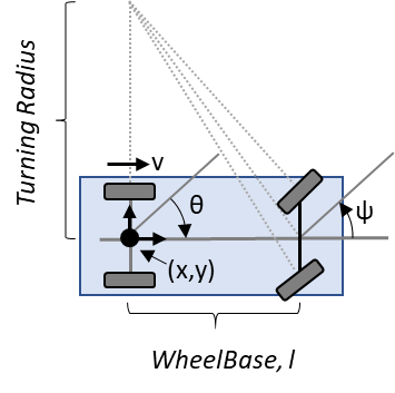
The Ackermann model state is [ $x$ $y$ $θ$ $ψ$ ].

Variables

$x$ : Global vehicle x-position in meters
$y$ : Global vehicle y-position in meters
$θ$ : Global vehicle heading in radians
$ψ$ : Vehicle steering angle in radians
$l$ : Wheel base in meters
$v$ : Vehicle speed in meters/s

Kinematic Equations

For the Ackermann kinematics model, the ODE is:

$[\begin{array}{cc} x_{}^{˙} \\ y_{}^{˙} \\ θ_{}^{˙} \\ ψ_{}^{˙} \end{array}] = [\begin{array}{cc} \cos (θ) & 0 \\ \sin (θ) & 0 \\ \tan (ψ) / l & 0 \\ 0 & 1 \end{array}] [\begin{array}{cc} v \\ ψ_{}^{˙} \end{array}]$

References

[1] Lynch, Kevin M., and Frank C. Park. Modern Robotics: Mechanics, Planning, and Control. Cambridge University Press, 2017.

For an example the simulates the different mobile robot using these models, see Simulate Different Kinematic Models for Mobile Robots.