Plan Paths with End-Effector Constraints Using State Spaces for Manipulators

Define State Space

To create a constrained state space, generate a class exampleHelperConstrainedStateSpace that derives from manipulatorStateSpace. Open this example to get the supporting file.

classdef exampleHelperConstrainedStateSpace < manipulatorStateSpace

Specify the constructor syntax which requires the robot model, end effector name, and target orientation as inputs. Define a property called EnableConstraint for turning the constraint on and off.

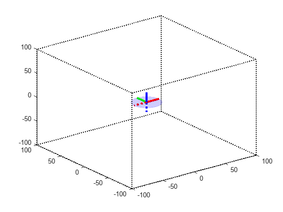
The constrained region is defined in the constructor using a workspaceGoalRegion object. The bounds on the xyz-position are all [-100,100] meters. The orientation bounds constrain the rotation about the z-axis to [-pi pi] with zero rotation about the x- and y-axes.

Create an inverse kinematics (IK) solver, and specify any solver parameters. This solver generates the joint configurations of the robot for the end-effector poses sampled inside the workspace.

        function obj = exampleHelperConstrainedStateSpace(rbt,endEffectorName,targetOrientation)
            %Constructor
            obj@manipulatorStateSpace(rbt);
            obj.EnableConstraint = true;
            obj.Region = workspaceGoalRegion(endEffectorName,'EndEffectorOffsetPose',targetOrientation);
            obj.Region.Bounds = [-100 100; -100 100; -100 100; -pi pi; 0 0; 0 0];
            
            % Store a reference of the manipulatorStateSpace/RigidBodyTree
            % in the Robot property. Note that the RigidBodyTree property
            % of the manipulatorStateSpace is read-only. Hence, accessing
            % it will involve creating a copy of the underlying handle,
            % which can be expensive.
            obj.Robot = obj.RigidBodyTree;
            
            % Configure the IK solver
            obj.IKSolver = inverseKinematics('RigidBodyTree', obj.Robot);
            obj.IKSolver.SolverParameters.AllowRandomRestart = false;
        end

Customize Interpolation Method

During the planning phase, the interpolate function connects configurations in the search tree. By default, the interpolation is unconstrained. Customize the interpolate function to ensure that the end-effector remains upright. Override the interpolate method on the manipulatorStateSpace object with this code.

        function constrainedStates = interpolate(obj, state1, state2, ratios)
            constrainedStates = interpolate@manipulatorStateSpace(obj,state1,state2,ratios);
            if(obj.EnableConstraint)
                for i = 1:size(constrainedStates, 1)
                    constrainedStates(i,:) = constrainConfig(obj,constrainedStates(i,:));
                end
            end
        end

The constraintConfig function replaces the unconstrained joint configurations with constrained configurations. It finds the end-effector pose closest to the constrained region [1] and returns the corresponding robot joint configuration. Given the end-effector pose ${\mathit{T}}_{\mathit{s}}^0$ corresponding to config, the function computes the pose closest to the end-effector pose in the constrained region and returns the corresponding robot joint configuration.

To find the closest pose in the reference frame, first find the displacement of ${\mathit{T}}_{\mathit{s}}^0$ from the region by calculating ${\mathit{T}}_{{\mathit{s}}^{\prime }}^{\mathit{w}}={{\mathit{T}}_{\mathit{w}}^0}^{-1}{\mathit{T}}_{\mathit{s}}^0{{\mathit{T}}_{\mathit{e}}^{\mathit{w}}}^{-1}$ and converting ${\mathit{T}}_{{\mathit{s}}^{\prime }}^{\mathit{w}}$ to a pose vector close to the bounds of the region. Given the bounds, there are three possibilities for an element in the pose vector and its corresponding bounds of the region:

Once the resulting closest constrained pose is found in the reference frame, convert this to a pose in the world coordinates.

        function constrainedConfig = constrainConfig(obj, config)
            %constrainConfig Constraint joint configuration to the region
            %   The function finds the joint configuration corresponding to
            %   the end-effector pose closest to the constrained region.
            wgr = obj.Region;
            T0_s = obj.Robot.getTransform(config, wgr.EndEffectorName);
            T0_w = wgr.ReferencePose;
            Tw_e = wgr.EndEffectorOffsetPose;
            Tw_sPrime = T0_w \ T0_s / Tw_e;
            dw = convertTransformToPoseVector(obj, Tw_sPrime);
            bounds = wgr.Bounds;
            
            % Find the pose vector closeset to the bounds of the region.
            for dofIdx = 1:6
                if(dw(dofIdx) < bounds(dofIdx, 1))
                    dw(dofIdx) = bounds(dofIdx, 1);
                elseif(dw(dofIdx) > bounds(dofIdx, 2))
                    dw(dofIdx) = bounds(dofIdx, 2);
                end
            end
            
            % Convert the pose vector in the region's reference frame to a
            % homogeneous transform.
            constrainedPose = obj.convertPoseVectorToTransform(dw);
            
            % Convert this pose to world coordinates, and find the
            % corresponding joint configuration.
            constrainedPose = T0_w * constrainedPose * Tw_e;
            constrainedConfig = obj.IKSolver(obj.Region.EndEffectorName, ...
                constrainedPose,  ...
                ones(1, 6), ...
                config);
        end

Create Robot State Space

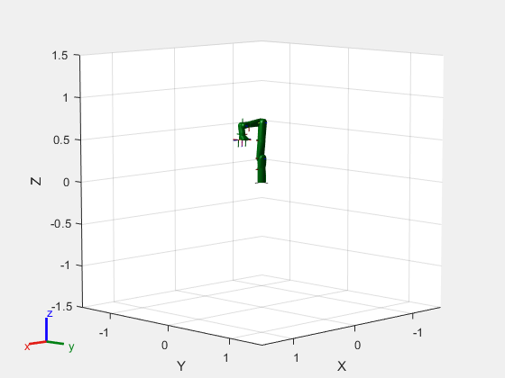
Now that you have setup your constrained state space, load an example robot and environment using the exampleHelperEndEffectorConstraintedEnvironment function. The output kinova is a rigid body tree robot model of the Kinova® Gen 3 and env is a cell array of collision body objects in the robot world.

[kinova,env] = exampleHelperEndEffectorConstrainedEnvironment;

Specify the end-effector name and target orientation. Store the joint position values for opening and closing the gripper.

endEffectorName = "EndEffector_Link";
targetOrientation = eul2tform([0 pi 0]);
openPostion = 0.06;
closedPosition = 0.04;

Create the customized state space.

ss = exampleHelperConstrainedStateSpace(kinova, endEffectorName, targetOrientation);

Specify state bounds on the gripper position so it remains open.

ss.StateBounds(end-1:end,:) = repmat([openPostion, openPostion], 2, 1);

Visualize the constrained workspaceGoalRegion region.

figure;
show(ss.Region)

Create State Validator

Create a manipulatorCollisionBodyValidator object from the state space and add the environment of collision objects. To improve performance, ignore self collisions when validating the state space. The robot model uses joint limits to ensure that self collisions will not occur.

sv = manipulatorCollisionBodyValidator(ss,"Environment",env,"SkippedSelfCollisions","parent");
sv.IgnoreSelfCollision = true;

Create Planner

This example uses the plannerBiRRT object, which is a bi-directional variant of the RRT algorithm with the "connect" heuristic enabled. For a sparse environment, this planner finds a solution in lesser number of iterations as compared to other RRT-based planners. Alternatively, for shorter paths with trimmed edges, consider the plannerRRTStar object.

The robot starts in a joint configuration which satisfies the constraint. Alternatively, the interpolate function of the constrained state space can be used to constrain the start configuration. This ensures that all the states in the resulting plan are constrained. Set the random number seed for repeatable results.

rng(20);
planner = plannerBiRRT(ss, sv);
planner.MaxConnectionDistance = 0.5;
planner.EnableConnectHeuristic = true;
startConfig = [0.1196 -0.045 -0.1303 1.6528 -0.0019 1.5032 0.0083, openPostion, openPostion];
figure("Visible","on");
show(kinova, startConfig, ...
    "Visuals", "off", ...
    "Collisions", "on", ...
    "PreservePlot", true);

Define Grasp Region

Next, define a grasping region using the workspaceGoalRegion object which represents a cylinder to pick in the environment (env{3}). Generate a joint configuration for a sampled end-effector pose. You should ensure that the configuration passed to the planner is collision-free.

graspingRegion = workspaceGoalRegion(endEffectorName);

% Attach the reference frame to the pose of the cylinder object.
graspingRegion.ReferencePose = env{3}.Pose;

% Define the offset of the end-effector relative to the target orientation.
graspingRegion.EndEffectorOffsetPose = trvec2tform([0, 0, 0.07]) * targetOrientation;

% Generate goal joint configuration of the robot given a sampled end-effector pose in
% the region.
goalConfig = jointConfigurationGiven(ss,sample(graspingRegion));
goalConfig(end-1:end) = openPostion;

Plan Path

Call the plan function to plan a path between the start and goal configurations. Time the planning phase. Interpolate the path to 50 points.

tic;
pickPath = plan(planner,startConfig,goalConfig);
tOut = toc;
interpolate(pickPath,50);
fprintf(newline);
fprintf("Planning finished in %d s\n", tOut);

Planning finished in 5.517940e-01 s

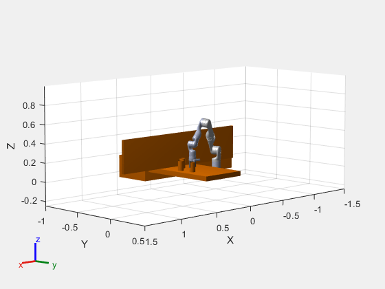
Visualize the planned path. The robot moves to the container to grab it.

hold on;
ylim([-1 0.5])
zlim([-0.25 1])
for i  = 1:length(env)
    show(env{i})
end
for i = 1:size(pickPath.States, 1)
    show(kinova, pickPath.States(i, :), ...
        "Visuals", "on", ...
        "FastUpdate",true, ...
        "Frames", "off", ...
        "PreservePlot",false);
    drawnow;
end
exampleHelperConstrainedRobotMoveGripper(kinova,...
    pickPath.States(end,:),openPostion,closedPosition);
hold off;

Recreate Planner

Attach the collision geometry of the can to the end-effector and remove the can from the environment. Then, with the modified robot, create a planning instance with the new robot model. After planning, you can deselect ss.EnableContraint and rerun this script to see a path without a constrained end effector.

zOffset = [0 0 (env{3}.Length)/2];
container = env{3};
addCollision(kinova.getBody(endEffectorName),env{3}, (env{3}.Pose) \ trvec2tform(zOffset));
env(3) = [];
ss = exampleHelperConstrainedStateSpace(kinova,endEffectorName,targetOrientation);

% Keep the end-effector closed during planning
ss.StateBounds(end-1:end,:) = repmat([0.04 0.04],2,1);
sv = manipulatorCollisionBodyValidator(ss, ...
    "Environment",env,"ValidationDistance",0.2,"SkippedSelfCollisions","parent");
planner = plannerBiRRT(ss,sv);
planner.MaxConnectionDistance = 1;
planner.EnableConnectHeuristic = true;

ss.EnableConstraint = true;

Plan Path

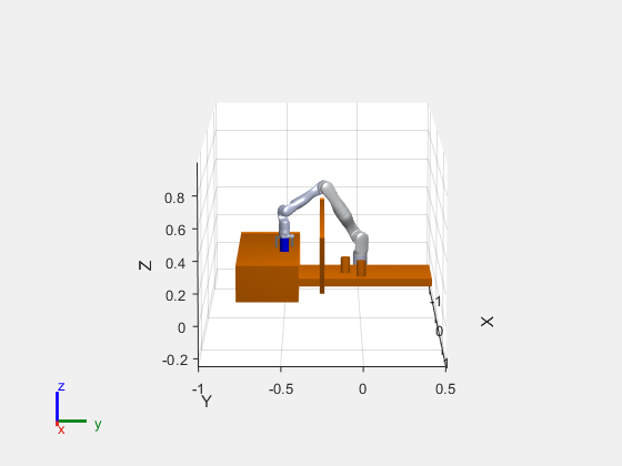
Next, plan from the last configuration in the previous path to a new goal joint configuration. The goal configuration places the can on the opposite table in the environment.

% The last state of the of the previous plan
startConfig = pickPath.States(end,:);
startConfig(end-1:end) = 0.04;
goalConfig = [1.1998 0.6044 0.0091 1.4219 -0.0058 1.1154 0.0076 0.04 0.04];
rng(10);
tic
placePath = plan(planner,startConfig,goalConfig);
tOut = toc;
fprintf("Planning finished in %0.2d s\n",tOut);

Planning finished in 1.86e+00 s

interpolate(placePath,50);

Visualize the path that places the container. Notice that the can remains upright throughout the path.

show(kinova, startConfig, ...
    "FastUpdate", false, ...
    "PreservePlot", false);
view([90,0,15])
ylim([-1 0.5])
zlim([-0.25 1])
hold on;
for i  = 1:length(env)
    show(env{i})
end
containerPose = hgtransform();
containerPose.Matrix = container.Pose;
[ax, p] = show(container);
p.FaceColor = [0 0 1];
p.Parent = containerPose;
for i = 1:size(placePath.States, 1)
    cPose = getTransform(kinova,placePath.States(i, :),endEffectorName);
    containerPose.Matrix = cPose/(container.Pose)*trvec2tform(zOffset);
    show(kinova,placePath.States(i,:), ...
        "FastUpdate",true, ...
        "PreservePlot",false, ...
        "Frames", "off");
    drawnow;
end
exampleHelperConstrainedRobotMoveGripper(kinova,...
    placePath.States(end,:),closedPosition,openPostion);
hold off;

Next Steps

To see an unconstrained path, deselect the ss.EnableConstraint check box and rerun the script. The cup tilts in a way that could easily spill the contents. You could also consider replacing the plannerBiRRT object with another sampling-based planner like plannerRRTStar to evaluate their performance.

References

[1] D. Berenson, S. Srinivasa, D. Ferguson, A. Collet, and J. Kuffner, "Manipulation Planning with Workspace Goal Regions", in Proceedings of IEEE International Conference on Robotics and Automation, 2009, pp.1397-1403