Survey Pit Mining Site with RTK GPS and Point Clouds
This example shows how to generate a digital elevation model (DEM) of a site using real-time kinematic (RTK) GPS and aerial lidar data.
While working on a site, periodic surveys are necessary to capture the latest features of the site map. One method to obtain this map involves using high-accuracy localization data from RTK GPS to stitch Lidar point clouds together. This example uses a UAV equipped with RTK GPS and a downward-facing lidar to survey a pit mine site and gather sensor data.
First, specify the parameters for the survey trajectory to ensure full coverage of the site.
Fs = 0.5; % Sampling rate (Hz)
uavSpeed = 10; % (m/s)
uavHeight = 300; % (m)
coverageAreaLength = 1100; % (m)
coverageAreaWidth = 1100; % (m)
unitLength = 10; % (m)
unitWidth = 200; % (m)
Define the coverage area of the site using the specified parameters and center it over the origin of the world frame.
coveragePolygon = [0 0; coverageAreaLength 0; coverageAreaLength coverageAreaWidth; 0 coverageAreaWidth];
coveragePolygon = coveragePolygon-[coverageAreaLength/2 coverageAreaWidth/2];
Use the survey parameters to create the coverage space, and then generate a coverage planner based on that space.
coverageSpace = uavCoverageSpace(Polygons=coveragePolygon, ...
    UnitLength=unitLength,UnitWidth=unitWidth,ReferenceHeight=uavHeight);
Create a coverage planner from the coverage space.
coveragePlanner = uavCoveragePlanner(coverageSpace,Solver="Exhaustive");Get the waypoints from the coverage planner.
takeoff = [0 0 0];
coverageWaypoints = plan(coveragePlanner,takeoff);
To ensure a straight flight between the waypoints, add extra waypoints to constrain the waypoint path. Also, remove the takeoff and landing waypoints because this example focuses on the waypoints in the air.
% Remove takeoff and landing waypoints.
coverageWaypoints = coverageWaypoints(2:end-1,:);

% To obtain a straight flight between waypoints, add extra waypoints to
% constrain the trajectory generation.
constrainedWaypoints = [];
diffWaypointsSign = sign(diff(coverageWaypoints));
for ii = 1:size(coverageWaypoints,1)-1
    constrainedWaypoints(end+1,:) = coverageWaypoints(ii,:); %#ok<SAGROW>
    if diffWaypointsSign(ii,1) ~= 0
        constrainedWaypoints(end+1,:) = coverageWaypoints(ii,:) ...
            + [diffWaypointsSign(ii,1) 0 0]; %#ok<SAGROW>
        constrainedWaypoints(end+1,:) = coverageWaypoints(ii+1,:) ...
            + [-diffWaypointsSign(ii,1) 0 0]; %#ok<SAGROW>
    end
end
Create a trajectory from the coverage waypoints and simulation parameters.
waypoints = constrainedWaypoints;
groundspeed = uavSpeed*ones(size(waypoints,1),1);
traj = waypointTrajectory(waypoints,GroundSpeed=groundspeed,SampleRate=Fs);
Get the UAV position and orientation from the trajectory generator.
t = traj.TimeOfArrival(1):(1/traj.SampleRate):traj.TimeOfArrival(end);
[uavPos,uavOrient] = lookupPose(traj,t);
View the coverage area and the generated trajectory.
figure
patch(coveragePolygon(:,1),coveragePolygon(:,2),"k",FaceAlpha=0.1)
hold on
plot(uavPos(:,1),uavPos(:,2),waypoints(:,1),waypoints(:,2)," o")
hold off
title("UAV Coverage Trajectory Above Site")
legend("Site Limits","Trajectory","Waypoints",Location="bestoutside")
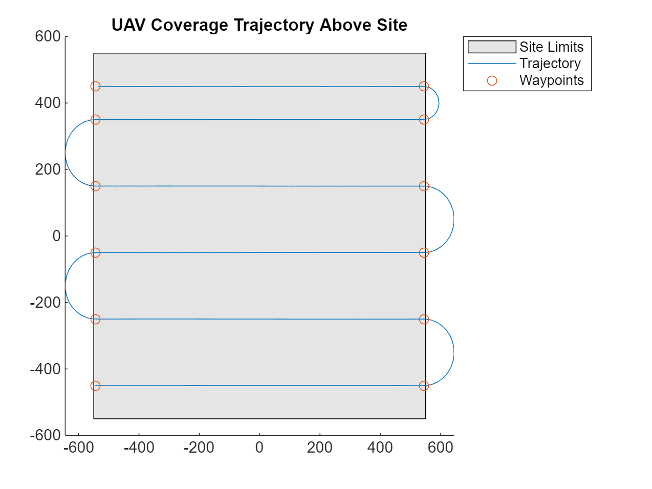
Store the trajectory and time parameters in a MAT-file. This MAT-file is used in the Simulink® model to collect the sensor data.
% Simulink model inputs and parameters.
uavPosition.time = t(:);
uavPosition.signals.values = permute(uavPos,[3 2 1]);
uavPosition.signals.dimensions = [1 3];

uavEulerAngles.time = t(:);
uavEulerAngles.signals.values = permute(euler(uavOrient,"ZYX","frame"),[3 2 1]);
uavEulerAngles.signals.dimensions = [1 3];

ts = 1/Fs;
simTime = t(end);

save("siteSurveyDataCollectionInputs.mat", ...
    "uavPosition","uavEulerAngles","ts","simTime");
Collect Sensor Data
Open the Simulink model containing scene setup and the UAV mounted with a GPS and lidar sensors.
model = "siteSurveyDataCollection";
open_system(model)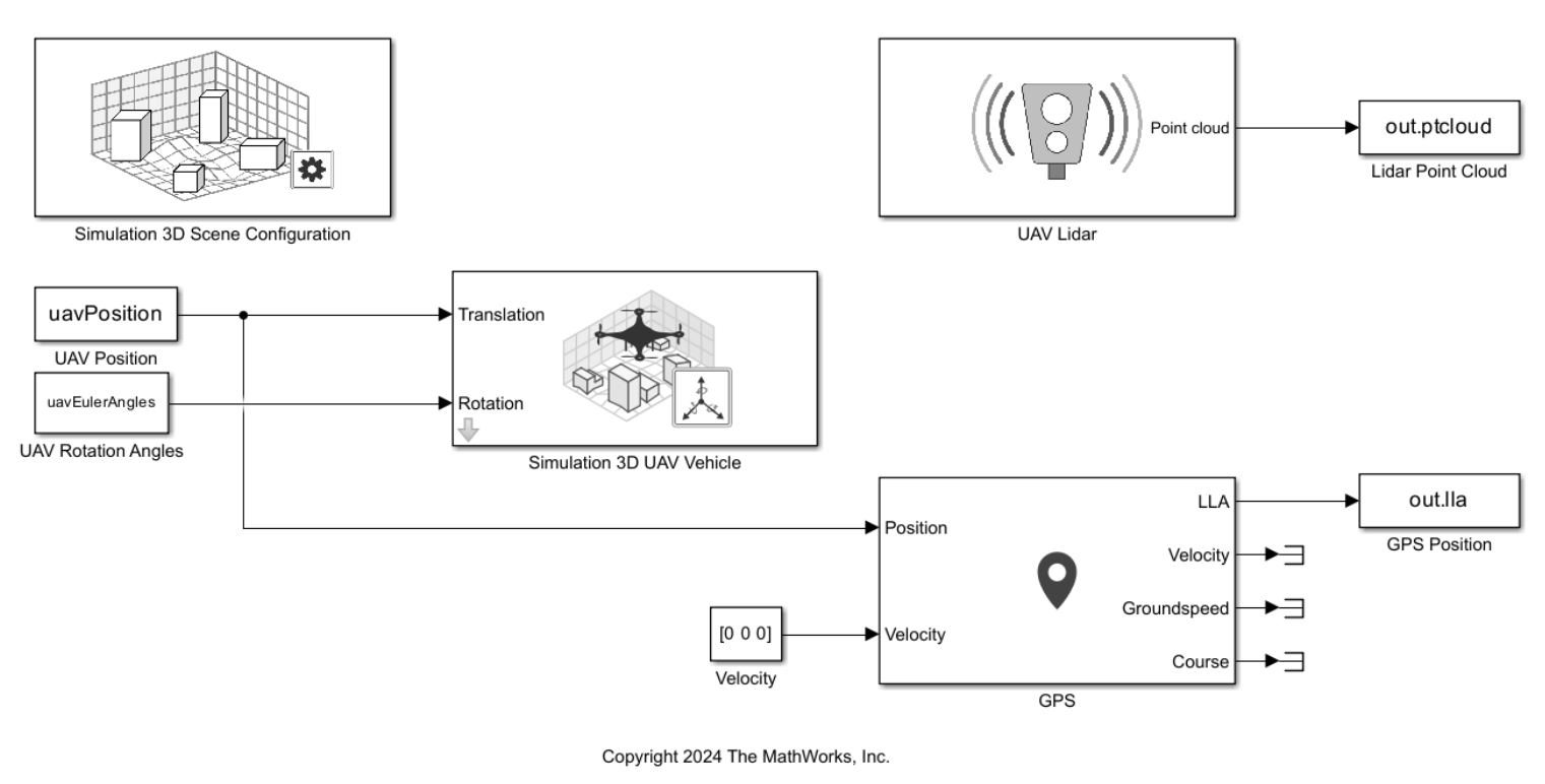
Open the Simulation 3D Scene Configuration block and set the Scene View parameter to Offroad pit mining scene. If you do not have this scene, see Offroad Pit Mining Scene for more information about how to download this scene.
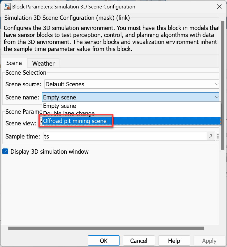
Run the model to collect the sensor data.
out = sim(model)
out =
  Simulink.SimulationOutput:

                    lla: [1x1 timeseries]
                ptcloud: [1x1 timeseries]
                   tout: [7941x1 double]

     SimulationMetadata: [1x1 Simulink.SimulationMetadata]
           ErrorMessage: [0x0 char]
This image shows the UAV surveying the pit mine scene with the lidar in the simulation.
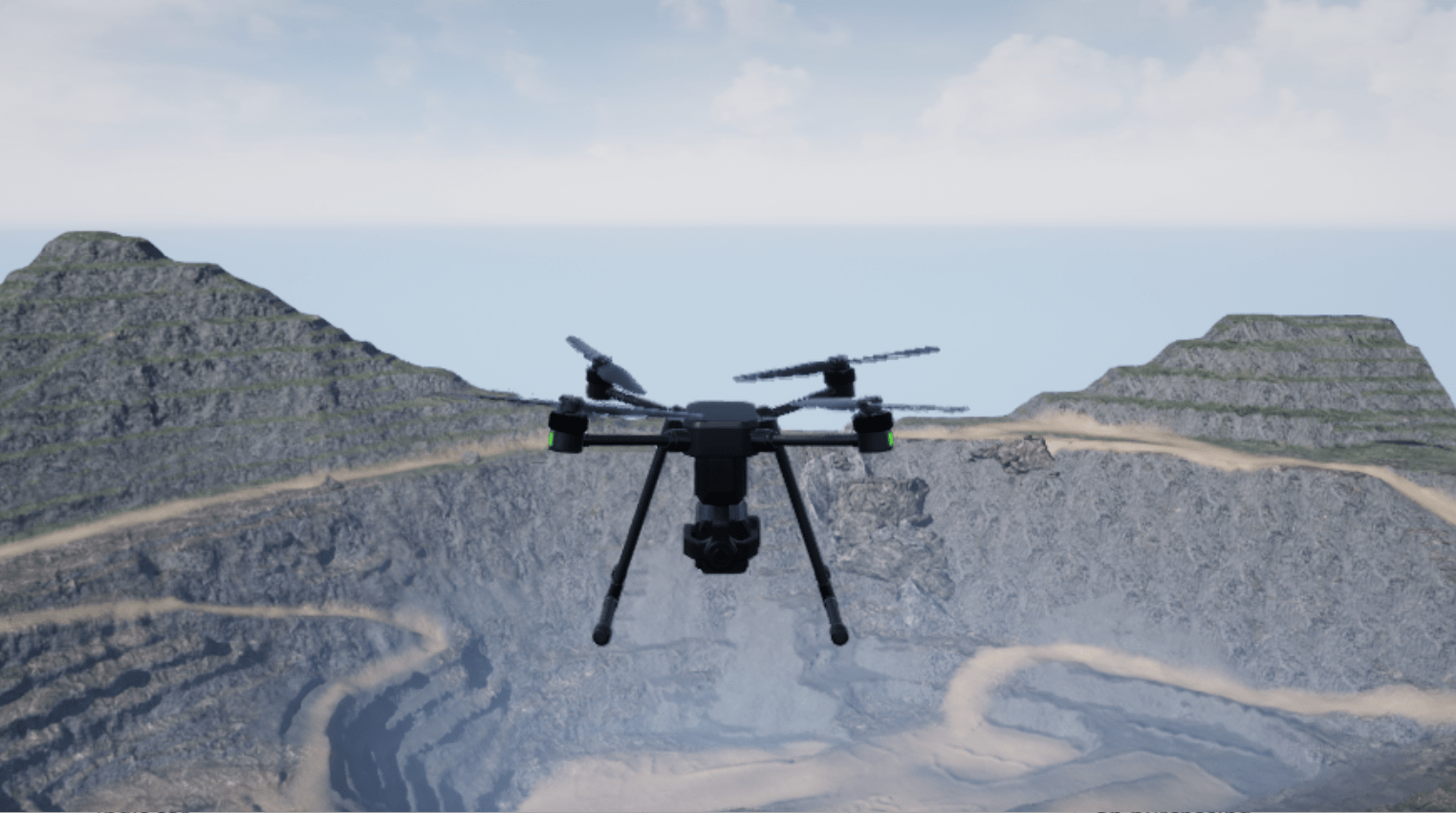
Convert Sensor Data to DEM
Extract the point cloud data.
ptclouds = out.ptcloud.Data;
Convert the GPS position to local Cartesian coordinates.
lla = permute(out.lla.Data,[3 2 1]);
lla0 = [0 0 0];
gpsPos = lla2enu(lla,lla0,"ellipsoid");
Get the orientation of the lidar relative to world coordinate system.
uavToLidarQuat = quaternion([0 90 0],'eulerd','zyx','frame');
worldToLidarRotMat = rotmat(uavOrient.*uavToLidarQuat,"frame");
Stitch the point cloud array using the UAV's RTK GPS and single receiver GPS readings, applying transformations to align each point cloud with the UAV and GPS positions.
gridStep = 0.1;
for ii = 2:size(ptclouds,4)
    % Determine the rotation matrix for the current lidar point cloud.
    R = worldToLidarRotMat(:,:,ii);

    % Create transformation objects for the UAV and GPS positions.
    tform = rigidtform3d(R.',uavPos(ii,:));
    tformGPS = rigidtform3d(R.',gpsPos(ii,:));

    % Apply the transformations to the current point cloud.
    ptCloudOut = pctransform(pointCloud(ptclouds(:,:,:,ii)),tform);
    ptCloudOutGPS = pctransform(pointCloud(ptclouds(:,:,:,ii)),tformGPS);

    % Merge the transformed point clouds with the accumulated point clouds.
    if ~(ii == 2)
        pcRTK = pcmerge(pcRTK,ptCloudOut,gridStep);
        pcGPS = pcmerge(pcGPS,ptCloudOutGPS,gridStep);
    else
        % Initialize the accumulated point clouds with the first transformed point cloud.
        pcRTK = ptCloudOut;
        pcGPS = ptCloudOutGPS;
    end
end
Generate the digital elevation models for the RTK GPS and single receiver GPS from the stitched point clouds.
terrainModelRTK = pc2dem(pcRTK);
terrainModelGPS = pc2dem(pcGPS);
Visualize DEM
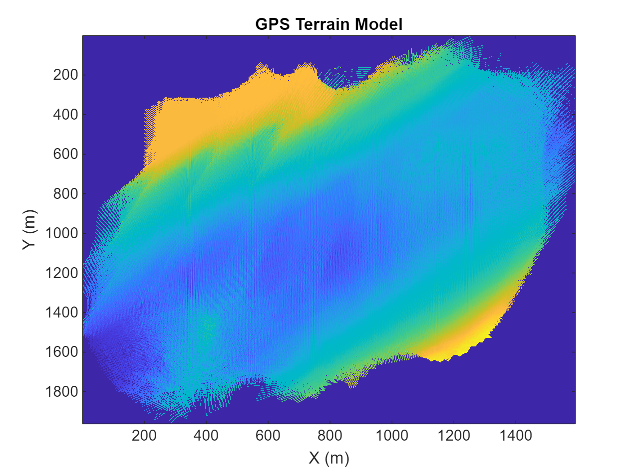
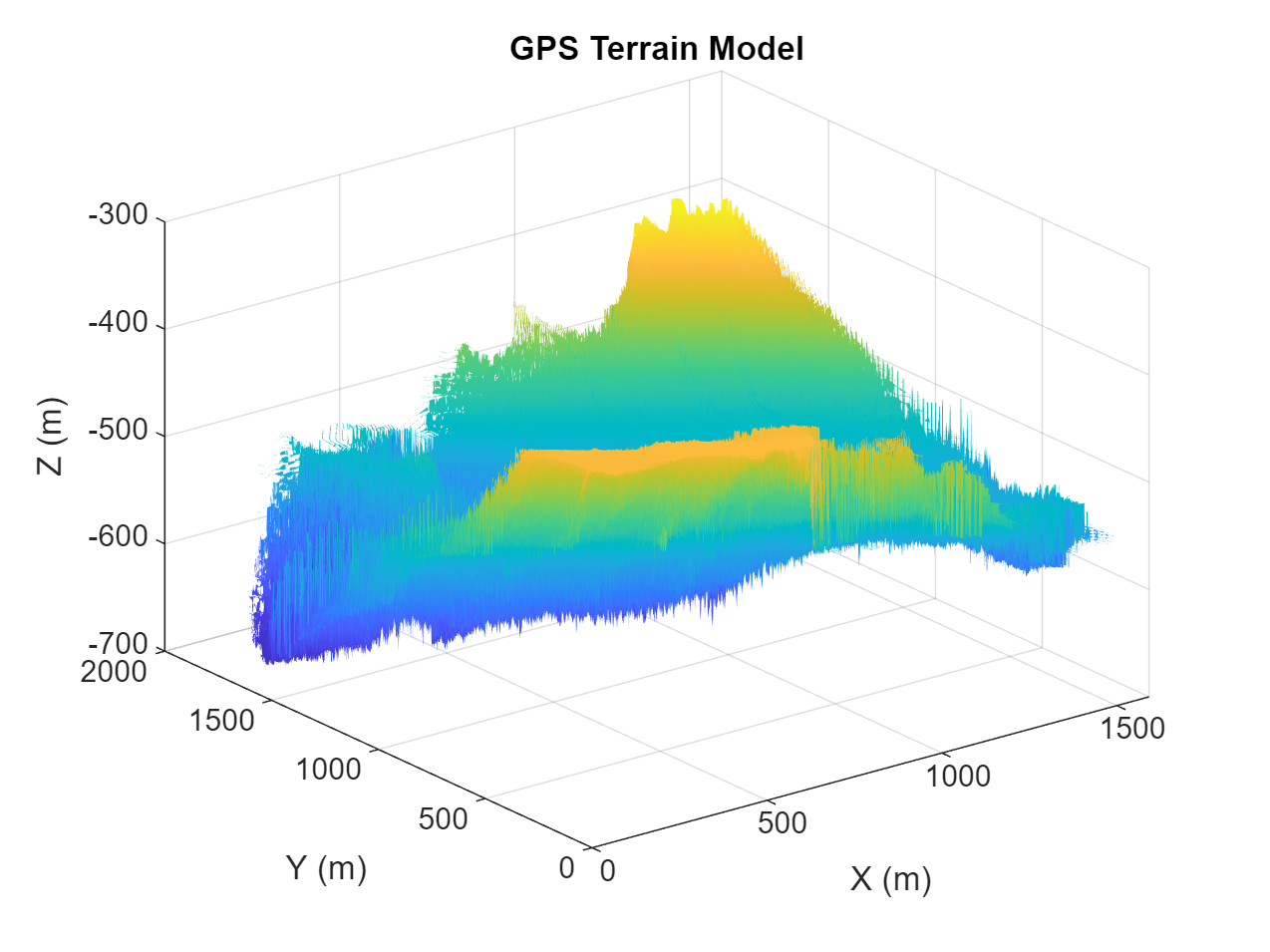
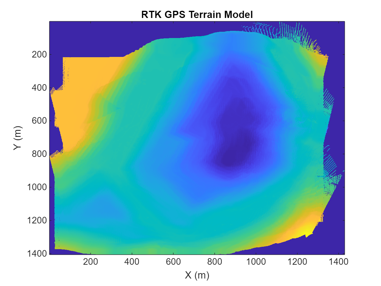
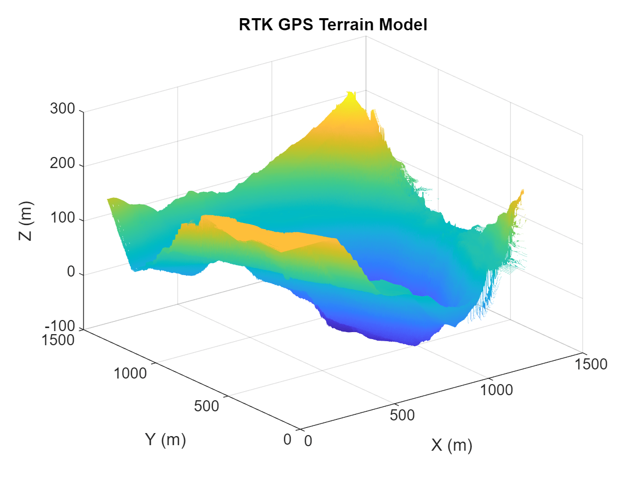
Plot the generated DEMs.
Note that due to the error in the single receiver GPS readings, the terrain model has overlapping sections, whereas the terrain model created from the RTK GPS readings has more smoother connected sections.
figure
imagesc(terrainModelGPS)
title("GPS Terrain Model")
xlabel("X (m)")
ylabel("Y (m)")
figure
surf(terrainModelGPS,EdgeColor="none")
title("GPS Terrain Model")
xlabel("X (m)")
ylabel("Y (m)")
zlabel("Z (m)")
figure
imagesc(terrainModelRTK)
title("RTK GPS Terrain Model")
xlabel("X (m)")
ylabel("Y (m)")
figure
surf(terrainModelRTK,EdgeColor="none")
title("RTK GPS Terrain Model")
xlabel("X (m)")
ylabel("Y (m)")
zlabel("Z (m)")
Conclusion
This example showed that you can use RTK GPS and lidar readings to create a site map, which is useful for sites that change over time like a pit mine. For sites where signal connection is unstable, you could instead use post-processing kinematic (PPK) GPS positioning. In this setup, the UAV logs only raw satellite observations rather than performing on-board RTK GPS positioning. The raw satellite observations are combined with a base station observation log file on a computer to obtain an accurate UAV position.