Fixed-Structure H-infinity Synthesis with hinfstruct

Introduction

The hinfstruct command extends classical $$H_{\infty }$$ synthesis (see hinfsyn) to fixed-structure control systems. This command is meant for users already comfortable with the hinfsyn workflow. If you are unfamiliar with $$H_{\infty }$$ synthesis or find augmented plants and weighting functions intimidating, use systune and looptune instead. See Tune Control Systems Using systune for the systune counterpart of this example.

Plant Model

This example uses a 9th-order model of the head-disk assembly (HDA) in a hard-disk drive. This model captures the first few flexible modes in the HDA.

load hinfstruct_demo G
bode(G), grid

We use the feedback loop shown below to position the head on the correct track. This control structure consists of a PI controller and a low-pass filter in the return path. The head position y should track a step change r with a response time of about one millisecond, little or no overshoot, and no steady-state error.

Figure 1: Control Structure

Tunable Elements

There are two tunable elements in the control structure of Figure 1: the PI controller $$C(s)$$ and the low-pass filter

Use the tunablePID class to parameterize the PI block and specify the filter $$F(s)$$ as a transfer function depending on a tunable real parameter $$a$$.

C0 = tunablePID('C','pi');  % tunable PI

a = realp('a',1);    % filter coefficient
F0 = tf(a,[1 a]);    % filter parameterized by a

Loop Shaping Design

Loop shaping is a frequency-domain technique for enforcing requirements on response speed, control bandwidth, roll-off, and steady state error. The idea is to specify a target gain profile or "loop shape" for the open-loop response $$L(s)=F(s)G(s)C(s)$$. A reasonable loop shape for this application should have integral action and a crossover frequency of about 1000 rad/s (the reciprocal of the desired response time of 0.001 seconds). This suggests the following loop shape:

wc = 1000;  % target crossover
s = tf('s');
LS = (1+0.001*s/wc)/(0.001+s/wc);
bodemag(LS,{1e1,1e5}), grid, title('Target loop shape')

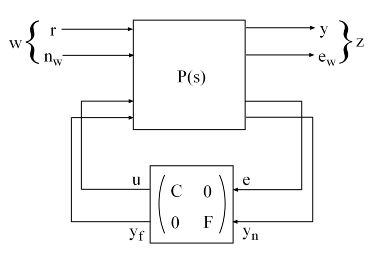
Note that we chose a bi-proper, bi-stable realization to avoid technical difficulties with marginally stable poles and improper inverses. In order to tune $$C(s)$$ and $$F(s)$$ with hinfstruct, we must turn this target loop shape into constraints on the closed-loop gains. A systematic way to go about this is to instrument the feedback loop as follows:

Figure 2: Closed-Loop Formulation

If $$T(s)$$ denotes the closed-loop transfer function from (r,nw) to (y,ew), the gain constraint

secures the following desirable properties:

We can therefore focus on tuning $$C(s)$$ and $$F(s)$$ to enforce $\Vert T{\Vert }_{\infty }<1$.

Specifying the Control Structure in MATLAB

In MATLAB®, you can use the connect command to model $$T(s)$$ by connecting the fixed and tunable components according to the block diagram of Figure 2:

% Label the block I/Os
Wn = 1/LS;  Wn.u = 'nw';  Wn.y = 'n';
We = LS;    We.u = 'e';   We.y = 'ew';
C0.u = 'e';   C0.y = 'u';
F0.u = 'yn';  F0.y = 'yf';

% Specify summing junctions
Sum1 = sumblk('e = r - yf');
Sum2 = sumblk('yn = y + n');

% Connect the blocks together
T0 = connect(G,Wn,We,C0,F0,Sum1,Sum2,{'r','nw'},{'y','ew'});

These commands construct a generalized state-space model T0 of $$T(s)$$. This model depends on the tunable blocks C and a:

T0.Blocks

ans = struct with fields:
    C: [1x1 tunablePID]
    a: [1x1 realp]

Note that T0 captures the following "Standard Form" of the block diagram of Figure 2 where the tunable components $$C,F$$ are separated from the fixed dynamics.

Figure 3: Standard Form for Disk-Drive Loop Shaping

Tuning the Controller Gains

We are now ready to use hinfstruct to tune the PI controller $$C$$ and filter $$F$$ for the control architecture of Figure 1. To mitigate the risk of local minima, run three optimizations, two of which are started from randomized initial values for C0 and F0.

rng('default')
opt = hinfstructOptions('Display','final','RandomStart',5);
T = hinfstruct(T0,opt);

Final: Peak gain = 3.88, Iterations = 67
Final: Peak gain = 597, Iterations = 190
       Some closed-loop poles are marginally stable (decay rate near 1e-07)
Final: Failed to enforce closed-loop stability (max Re(s) = -1e-07)
Final: Peak gain = 3.88, Iterations = 68
Final: Peak gain = 1.56, Iterations = 98
Final: Peak gain = 1.56, Iterations = 99

The best closed-loop gain is 1.56, so the constraint $\Vert T{\Vert }_{\infty }<1$ is nearly satisfied. The hinfstruct command returns the tuned closed-loop transfer $$T(s)$$. Use showTunable to see the tuned values of $$C$$ and the filter coefficient $$a$$:

showTunable(T)

C =
 
             1 
  Kp + Ki * ---
             s 

  with Kp = 0.000846, Ki = 0.0103
 
Name: C
Continuous-time PI controller in parallel form.
-----------------------------------
a = 5.49e+03

Use getBlockValue to get the tuned value of $$C(s)$$ and use getValue to evaluate the filter $$F(s)$$ for the tuned value of $$a$$:

C = getBlockValue(T,'C');
F = getValue(F0,T.Blocks);  % propagate tuned parameters from T to F

tf(F)

ans =
 
  From input "yn" to output "yf":
    5486
  --------
  s + 5486
 
Continuous-time transfer function.

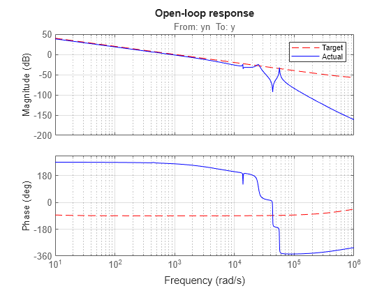
To validate the design, plot the open-loop response L=F*G*C and compare with the target loop shape LS:

bode(LS,'r--',G*C*F,'b',{1e1,1e6}), grid, 
title('Open-loop response'), legend('Target','Actual')

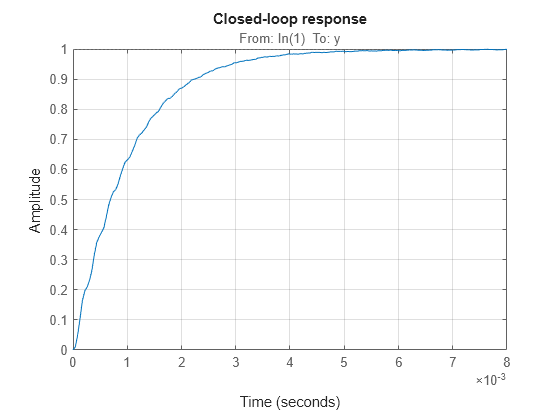
The 0dB crossover frequency and overall loop shape are as expected. The stability margins can be read off the plot by right-clicking and selecting the Characteristics menu. This design has 24dB gain margin and 81 degrees phase margin. Plot the closed-loop step response from reference r to position y:

step(feedback(G*C,F)), grid, title('Closed-loop response')

While the response has no overshoot, there is some residual wobble due to the first resonant peaks in G. You might consider adding a notch filter in the forward path to remove the influence of these modes.

Tuning the Controller Gains from Simulink

Suppose you used this Simulink model to represent the control structure. If you have Simulink® Control Design™ installed, you can tune the controller gains from this Simulink model as follows. First mark the signals r,e,y,n as Linear Analysis points in the Simulink model.

Then create an instance of the slTuner interface and mark the Simulink blocks C and F as tunable:

ST0 = slTuner('rct_diskdrive',{'C','F'});

Since the filter $$F(s)$$ has a special structure, explicitly specify how to parameterize the F block:

a = realp('a',1);    % filter coefficient
setBlockParam(ST0,'F',tf(a,[1 a]));

Finally, use getIOTransfer to derive a tunable model of the closed-loop transfer function $$T(s)$$ (see Figure 2)

% Compute tunable model of closed-loop transfer (r,n) -> (y,e)
T0 = getIOTransfer(ST0,{'r','n'},{'y','e'});

% Add weighting functions in n and e channels
T0 = blkdiag(1,LS) * T0 * blkdiag(1,1/LS);

You are now ready to tune the controller gains with hinfstruct:

rng(0)
opt = hinfstructOptions('Display','final','RandomStart',5);
T = hinfstruct(T0,opt);

Final: Peak gain = 3.88, Iterations = 67
Final: Peak gain = 597, Iterations = 190
       Some closed-loop poles are marginally stable (decay rate near 1e-07)
Final: Peak gain = 596, Iterations = 161
       Some closed-loop poles are marginally stable (decay rate near 1e-07)
Final: Peak gain = 3.88, Iterations = 70
Final: Peak gain = 1.56, Iterations = 99
Final: Peak gain = 1.56, Iterations = 99

Verify that you obtain the same tuned values as with the MATLAB approach:

showTunable(T)

C =
 
             1 
  Kp + Ki * ---
             s 

  with Kp = 0.000846, Ki = 0.0103
 
Name: C
Continuous-time PI controller in parallel form.
-----------------------------------
a = 5.49e+03