Robust Controller Design

Design Controller

Because of the nominal first-order behavior of the plant, choose a PI control architecture. For a desired closed-loop damping ratio ξ and natural frequency ${\omega }_{\mathit{n}}$, the design equations for the proportional and integral gains (based on the nominal open-loop time constant of 0.2) are:

To study how the uncertainty in G affects the achievable closed-loop bandwidth, design two controllers, both achieving ξ = 0.707, but with different ${\omega }_{\mathit{n}}$ values, 3 and 7.5.

xi = 0.707;
wn1 = 3;
wn2 = 7.5; 

Kp1 = 2*xi*wn1/5 - 1;
Ki1 = (wn1^2)/5;
C1 = tf([Kp1,Ki1],[1 0]);

Kp2 = 2*xi*wn2/5 - 1;
Ki2 = (wn2^2)/5;
C2 = tf([Kp2,Ki2],[1 0]);

Examine Controller Performance

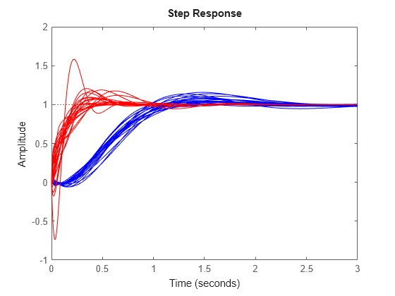
The nominal closed-loop bandwidth achieved by C2 is in a region where G has significant model uncertainty. It is therefore expected that the model variations cause significant degradations in the closed-loop performance with that controller. To examine the performance, form the closed-loop systems and plot the step responses of samples of the resulting systems.

T1 = feedback(G*C1,1);
T2 = feedback(G*C2,1);
tfinal = 3;
step(T1,'b',T2,'r',tfinal)

The step responses for T2 exhibit a faster rise time because C2 sets a higher closed-loop bandwidth. However, as expected, the model variations have a greater impact.

You can use robstab to check the robustness of the stability of the closed-loop systems to model variations.

opt = robOptions('Display','on');
stabmarg1 = robstab(T1,opt);

Computing peak...  Percent completed: 100/100
System is robustly stable for the modeled uncertainty.
 -- It can tolerate up to 401% of the modeled uncertainty.
 -- There is a destabilizing perturbation amounting to 401% of the modeled uncertainty.
 -- This perturbation causes an instability at the frequency 3.74 rad/seconds.

stabmarg2 = robstab(T2,opt);

Computing peak...  Percent completed: 100/100
System is robustly stable for the modeled uncertainty.
 -- It can tolerate up to 125% of the modeled uncertainty.
 -- There is a destabilizing perturbation amounting to 125% of the modeled uncertainty.
 -- This perturbation causes an instability at the frequency 11.4 rad/seconds.

The display gives the amount of uncertainty that the system can tolerate without going unstable. In both cases, the closed-loop systems can tolerate more than 100% of the modeled uncertainty range while remaining stable. stabmarg contains lower and upper bounds on the stability margin. A stability margin greater than 1 means the system is stable for all values of the modeled uncertainty. A stability margin less than 1 means there are allowable values of the uncertain elements that make the system unstable.

Compare Nominal and Worst-Case Behavior

While both systems are stable for all variations, their performance is affected to different degrees. To determine how the uncertainty affects closed-loop performance, you can use wcgain to compute the worst-case effect of the uncertainty on the peak magnitude of the closed-loop sensitivity function, S = 1/(1+GC). This peak gain of this function is typically correlated with the amount of overshoot in a step response; peak gain greater than one indicates overshoot.

Form the closed-loop sensitivity functions and call wcgain.

S1 = feedback(1,G*C1);
S2 = feedback(1,G*C2);
[maxgain1,wcu1] = wcgain(S1);
[maxgain2,wcu2] = wcgain(S2);

maxgain gives lower and upper bounds on the worst-case peak gain of the sensitivity transfer function, as well as the specific frequency where the maximum gain occurs. Examine the bounds on the worst-case gain for both systems.

maxgain1

maxgain1 = struct with fields:
           LowerBound: 1.8831
           UpperBound: 1.8861
    CriticalFrequency: 3.1938

maxgain2

maxgain2 = struct with fields:
           LowerBound: 4.6286
           UpperBound: 4.6378
    CriticalFrequency: 11.6132

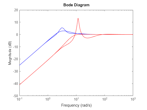
wcu contains the particular values of the uncertain elements that achieve this worst-case behavior. Use usubs to substitute these worst-case values for uncertain elements, and compare the nominal and worst-case behavior.

wcS1 = usubs(S1,wcu1);
wcS2 = usubs(S2,wcu2);
bodemag(S1.NominalValue,'b',wcS1,'b');
hold on
bodemag(S2.NominalValue,'r',wcS2,'r');

While C2 achieves better nominal sensitivity than C1, the nominal closed-loop bandwidth extends too far into the frequency range where the process uncertainty is very large. Hence the worst-case performance of C2 is inferior to C1 for this particular uncertain model.