Main Content

fitmagfrd

Fit frequency response magnitude data with minimum-phase state-space model using log-Chebyshev magnitude design

Description

B = fitmagfrd(A,N) computes a stable, minimum-phase state-space model of order N with a frequency response that approximates the frequency-response model A.

example

B = fitmagfrd(A,N,RD) forces the relative degree of B to RD. The relative degree of B is the difference between the number of poles and the number of zeros of B.

B = fitmagfrd(A,N,RD,WT) uses the magnitude of WT to weight the optimization fit criteria. Use WT to give greater weight to matching the responses of B and A at certain frequencies.

B = fitmagfrd(A,N,RD,WT,C) enforces additional constraints on the magnitude of B.

example

Examples

collapse all

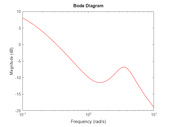
Create frequency response magnitude data from a fifth-order system.

sys = tf([1 2 2],[1 2.5 1.5])*tf(1,[1 0.1]); 
sys = sys*tf([1 3.75 3.5],[1 2.5 13]); 
omega = logspace(-1,1); 
sysg = abs(frd(sys,omega)); 
bodemag(sysg,'r');

MATLAB figure

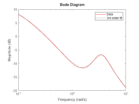
Fit the magnitude data with a minimum-phase, stable third-order system.

ord = 3; 
b1 = fitmagfrd(sysg,ord); 
b1g = frd(b1,omega); 
bodemag(sysg,'r',b1g,'k:');
legend('Data','3rd order fit');

MATLAB figure

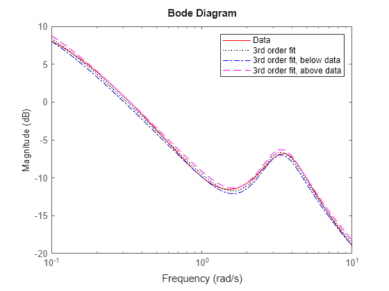
Fit the magnitude data with a third-order system constrained to lie below and above the given data.

C2.UpperBound = sysg;
C2.LowerBound = [];
b2 = fitmagfrd(sysg,ord,[],[],C2); 
b2g = frd(b2,omega); 
C3.UpperBound = [];
C3.LowerBound = sysg;
b3 = fitmagfrd(sysg,ord,[],[],C3); 
b3g = frd(b3,omega); 
bodemag(sysg,'r',b1g,'k:',b2g,'b-.',b3g,'m--') 
legend('Data','3rd order fit','3rd order fit, below data',...
       '3rd order fit, above data')

MATLAB figure

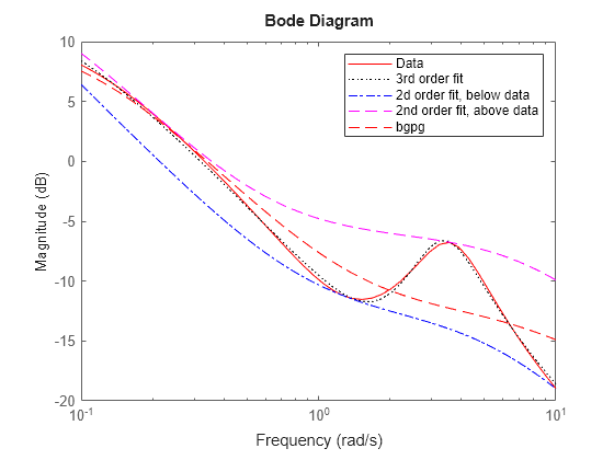
Fit the magnitude data with a second-order system constrained to lie below and above the given data.

ord = 2;
C2.UpperBound = sysg;
C2.LowerBound = [];
b2 = fitmagfrd(sysg,ord,[],sysg,C2);
b2g = frd(b2,omega);
C3.UpperBound = [];
C3.LowerBound = sysg;
b3 = fitmagfrd(sysg,ord,[],sysg,C3);
b3g = frd(b3,omega);
bgp = fitfrd(genphase(sysg),ord);
bgpg = frd(bgp,omega);
bodemag(sysg,'r',b1g,'k:',b2g,'b-.',b3g,'m--',bgpg,'r--')
legend('Data','3rd order fit','2d order fit, below data',...
       '2nd order fit, above data','bgpg')

MATLAB figure

Input Arguments

collapse all

Frequency response data, specified as an frd model. A must be SISO, have a single input with multiple outputs, or have multiple outputs with a single input.

Order of output model B, specified as a nonnegative integer. Numerical conditioning problems arise if the specified N is higher than required by the dynamics of A.

Relative degree, specified as a nonnegative integer. The default value for RD is 0. You can specify the default value for RD by setting RD to an empty matrix.

Weight, specified as an array, ss model, orfrd model. If WT is a scalar, then it is used to weight all entries of the error criteria (A-B). If WT is a vector, it must be the same size as A, and each individual entry of WT acts as a weighting function on the corresponding entry of (A-B).

Additional constraints on the magnitude of B, specified as:

  • A structure with fields C.LowerBound and C.UpperBound, specifying lower bounds and upper bounds on the magnitude of B. Specify the value of each field as a numeric array or an frd model of the same size as A, giving the target bound on the magnitude at each frequency. To enforce only a lower bound, set C.UpperBound = Inf. Similar, to enforce only an upper bound, set C.LowerBound = -Inf.

  • An array of the same size as A.Frequency or an frd model with C.Frequency = A.Frequency, then the upper and lower bounds on B are as follows.

    • If C(w) == –1, then enforce abs(B(w)) <= abs(A(w)).

    • if C(w) == 1, then enforce abs(B(w)) >= abs(A(w)).

    • if C(w) == 0, then no additional constraint at frequency w.

Output Arguments

collapse all

Fit for the input frequency-response data, returned as a stable, minimum-phase state-space (ss) model. B has order N and the same size as A.

Algorithms

fitmagfrd uses a version of log-Chebyshev magnitude design, solving

   min f     subject to (at every frequency point in A):  
           |d|^2 /(1+ f/WT) < |n|^2/A^2 < |d|^2*(1 + f/WT) 

plus additional constraints imposed with C. Here n and ddenote the numerator and denominator, respectively, and B = n/d. n and d have orders (N-RD) and N, respectively. The problem is solved using linear programming for fixed f and bisection to minimize f. An alternate approximate method, which cannot enforce the constraints defined by C, is B = fitfrd(genphase(A),N,RD,WT).

References

[1] Oppenheim, A.V., and R.W. Schaffer, Digital Signal Processing, Prentice Hall, New Jersey, 1975, p. 513.

[2] Boyd, S. and Vandenberghe, L., Convex Optimization, Cambridge University Press, 2004.

Version History

Introduced before R2006a
See Also

Go to top of page