Disk Margin and Smallest Destabilizing Perturbation

Disk Margin as Range of Allowable Gain and Phase Variations

Compute the disk margins of a SISO feedback loop with open-loop response L.

L = tf(25,[1 10 10 10]);
DM = diskmargin(L);

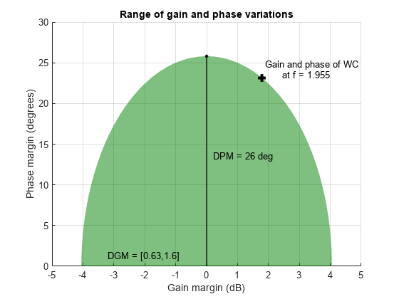
The disk-based margins define a range of "safe" gain and phase variations for which the feedback loop remains stable. The diskmarginplot command lets you visualize this range as a region in the gain-phase plane. As long as gain and phase variations stay within the shaded region, the closed-loop system feedback(L,1) remains stable.

diskmarginplot(DM.GainMargin)

diskmargin models gain and phase variations as a complex-valued multiplicative factor F applied to the nominal loop transfer L. The set of F values is a disk whose intersection with the real axis is the interval DM.GainMargin. (See Stability Analysis Using Disk Margins.) diskmarginplot can also plot the F disk.

diskmarginplot(DM.GainMargin,'disk')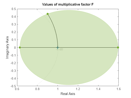

diskmargin also computes the smallest variation that destabilizes the feedback loop, returned in the field DM.WorstPerturbation. This variation is returned as a state-space model that realizes the destabilizing gain and phase variation. When you multiply L by this perturbation, the resulting closed-loop system has an undamped pole at the frequency returned in DM.Frequency.

WC = DM.WorstPerturbation;
CL = feedback(L*WC,1);
damp(CL)

                                                                       
         Pole              Damping       Frequency      Time Constant  
                                       (rad/seconds)      (seconds)    
                                                                       
 -1.49e+00 + 7.93e-01i     8.83e-01       1.69e+00         6.70e-01    
 -1.49e+00 - 7.93e-01i     8.83e-01       1.69e+00         6.70e-01    
  5.55e-16 + 1.96e+00i    -2.84e-16       1.96e+00        -1.80e+15    
  5.55e-16 - 1.96e+00i    -2.84e-16       1.96e+00        -1.80e+15    
 -4.19e+00                 1.00e+00       4.19e+00         2.39e-01    
 -9.46e+00                 1.00e+00       9.46e+00         1.06e-01    

Verify that the gain and phase variation of the destabilizing perturbation mark a boundary point for the range of "safe" gain and phase variations. To do so, compute the gain and phase of WC at DM.Frequency.

hWC = freqresp(WC,DM.Frequency);

GM = mag2db(abs(hWC))

GM = 
1.7832

PM = 180/pi * abs(angle(hWC))

PM = 
23.1695

diskmarginplot(DM.GainMargin)
line(GM,PM,'Color','k','Marker','+','MarkerSize',8,'LineWidth',3,'HandleVisibility','off')
text(GM+.1,PM+1,sprintf('Gain and phase of WC\n      at f = %.5g',DM.Frequency))

Nyquist Interpretation

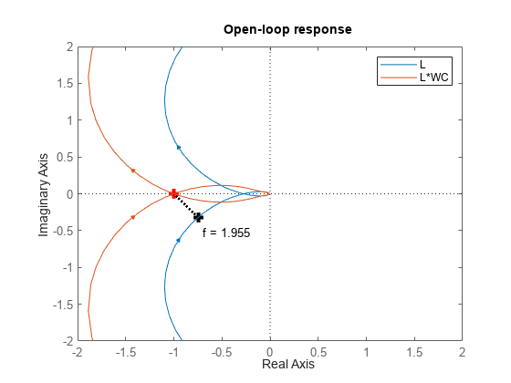
The statement that the perturbation WC drives the closed-loop system unstable is equivalent to saying that the Nyquist plot of L*WC touches the critical point at the frequency DM.Frequency. (See Stability Analysis Using Disk Margins.) The following plot shows the Nyquist plots of L and L*WC. The crosses on each plot mark the response at DM.Frequency, and confirm that the response of L*WC is –1 at this frequency.

figure(2), clf
hL = freqresp(L,DM.Frequency);
nyquist(L,L*WC)
title('Open-loop response')
legend('L','L*WC');
axis([-2 2 -2 2])
line(-1,0,'Color','r','Marker','+','MarkerSize',8,...
          'LineWidth',3,'HandleVisibility','off')
line(real(hL),imag(hL),'Color','k','Marker','+',...
          'MarkerSize',8,'LineWidth',3,'HandleVisibility','off')
text(real(hL)+0.05,imag(hL)-0.2,sprintf('f = %.5g',DM.Frequency))
line([real(hL) -1],[imag(hL) 0],'Color','k','LineStyle',':',...
          'LineWidth',2,'HandleVisibility','off')

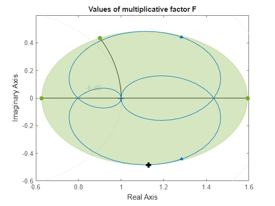
The perturbation WC is dynamic and its Nyquist plot hugs the boundary of the disk of F values. The point of contact is the frequency DM.Frequency where the disk margin is weakest. The following plot uses diskmarginplot to render the disk of allowable gain and phase variations on the Nyquist plane, superimposing the response of the perturbation WC. The black cross again marks the response at DM.Frequency.

hWC = freqresp(WC,DM.Frequency);

diskmarginplot(DM.GainMargin,'disk')
hold on
nyquist(WC)
hold off
axis([0.6 1.6 -0.6 0.6])
line(real(hWC),imag(hWC),'Color','k','Marker','+',...
   'MarkerSize',8,'LineWidth',3,'HandleVisibility','off')
text(real(hWC)+0.02,imag(hWC)-0.05,sprintf('f = %.5g',DM.Frequency))

Equivalently, this frequency is where the Nyquist plot of L touches the exclusion region associated with the disk margins DM. The following plot shows the disk of variations with the Nyquist plot of L. The black cross marks the response of L at DM.Frequency.

diskmarginplot(DM.GainMargin,'nyquist')
hold on
nyquist(L)
hold off
axis([-2 0 -1 1])
line(real(hL),-imag(hL),'Color','k','Marker','+',...
        'MarkerSize',8,'LineWidth',3,'HandleVisibility','off')
text(real(hL)+0.05,-imag(hL)+0.05,sprintf('f = %.5g',DM.Frequency))

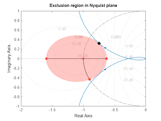
Thus, the disk F represents a region in the Nyquist plane that the response of L cannot enter while preserving closed-loop stability. At the critical frequency DM.Frequency, the frequency at which the gain and phase margins are smallest, the Nyquist plot of L just touches the disk.