diskmarginplot

Visualize disk-based stability margins

Since R2020a

collapse all in page

Syntax

diskmarginplot(L)

diskmarginplot(L1,...,LN)

diskmarginplot(L1,LineSpec1,...,LN,LineSpecN)

diskmarginplot(___,sigma)

diskmarginplot(___,w)

diskmarginplot(___,opts)

diskmarginplot(DGM)

diskmarginplot(DGM,'disk')

diskmarginplot(DGM,'nyquist')

diskmarginplot(alpha,sigma,___)

diskmarginplot(AX,___)

Description

Margins as a Function of Frequency

diskmarginplot(L) plots the disk-based gain and phase margins for the SISO or MIMO negative feedback loop feedback(L,eye(N)), where N is the number of inputs and outputs in the open-loop response L.

For MIMO responses, diskmarginplot plots the multiloop disk margins. The disk-based gain margin at each frequency is ±GM, where GM is the value shown in the plot in dB. Similarly, the disk-based phase margin is ±PM degrees, where PM is the value shown on the plot. For details about disk-based gain and phase margins, see diskmargin.

example

diskmarginplot(L1,...,LN) plots the disk-based gain and phase margins of multiple open-loop responses on the same plot.

example

diskmarginplot(L1,LineSpec1,...,LN,LineSpecN) specifies a color, line style, and marker for each system in the plot.

example

diskmarginplot(___,sigma) plots the disk-based gain and phase margins computed using the skew sigma to bias the gain variation toward gain increase (sigma > 0) or gain decrease (sigma < 0). If you have used diskmargin to obtain disk-based margins with some particular sigma, you can use this syntax to see the frequency dependence of the margins at that sigma value. For sigma ≠ 0, the plotted value is GM = min(gmax,1/max(0,gmin)). In other words, the plot shows the largest amount of gain change [1/GM,GM] that fits within the disk-based gain margin [gmin,gmax] of the system at the specified sigma.

diskmarginplot(___,w) plots the margins at the frequencies specified by w.

If w is a cell array of the form {wmin,wmax}, then the plot shows the margins at frequencies ranging between wmin and wmax.
If w is a vector of frequencies, then the plot shows the margins at each specified frequency.

diskmarginplot(___,opts) uses specified options to customize plot elements such as labels, ticks, and grids. You can use this argument with any of the previous syntaxes.

example

Range of Gain and Phase Variations

diskmarginplot(DGM) plots the range of simultaneous gain and phase variations corresponding to a disk-based gain margin. The plot also shows the maximum gain-only and phase-only variations (this disk-based gain and phase margins). DGM is a vector of the form [gmin,gmax]. The gain margin DGM can also be a scalar, which is equivalent to specifying the symmetric gain variation [1/DGM,DGM]. To plot the ranges for multiple disk-based gain margins at once, use a two-column matrix of the form [gmin1,gmax1;...;gminN,gmaxN]. For more information about disk-based gain margins, see diskmargin.

example

diskmarginplot(DGM,'disk') plots the complex-valued disk of modeled gain and phase variations corresponding to the disk-based gain margin DGM. For details about how disk-margin analysis models gain and phase variations, see Stability Analysis Using Disk Margins.

example

diskmarginplot(DGM,'nyquist') plots the exclusion region in the Nyquist plane corresponding to the disk margin DGM. The requirement that the closed-loop system remain stable for gain or phase variations within the disk corresponding to DGM amounts to a requirement that the open-loop response remain outside a disk-shaped exclusion region in the Nyquist plane. For more information, see Stability Analysis Using Disk Margins.

example

diskmarginplot(alpha,sigma,___) plots the range of gain and phase variations corresponding to the disk size alpha and skew sigma. If either alpha or sigma is a vector, then the plot includes the ranges for all specified values. If both alpha and sigma are vectors, then the plot includes the ranges for the pairs alpha1,sigma1;...;alphaN,sigmaN.

To plot the modeled uncertainty disk corresponding to alpha,sigma, use this syntax with the 'disk' flag. To plot the corresponding exclusion disk in the Nyquist plane, use this syntax with the 'nyquist' flag.

example

Plot on Specified Axes

diskmarginplot(AX,___) draws a plot on the axes specified by an axes handle (axes or a UIaxes object). Use this argument to specify axes when creating apps in Develop Apps Using App Designer. You can use this argument with any of the previous syntaxes to draw any of the plots that diskmarginplot can generate.

Examples

collapse all

Plot Gain and Phase Margins Versus Frequency

Open Live Script

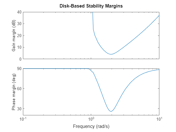
Plot the disk-based gain and phase margins of a system with open loop response L and closed-loop response feedback(L,1).

L = tf(25,[1 10 10 10]);
diskmarginplot(L)

MATLAB figure

The disk-based gain margin at each frequency is at least ±GM, where GM is the value shown in the plot in dB. Similarly, the disk-based phase margin is ±PM degrees. The disk-based margins returned by the diskmargin command are the smallest margins over frequency. (Right-click on the plot and select Characteristics > Minimum Disk Margin for a data tip containing information about these minimum margins.)

Compare Disk Margins of Multiple Systems

Open Live Script

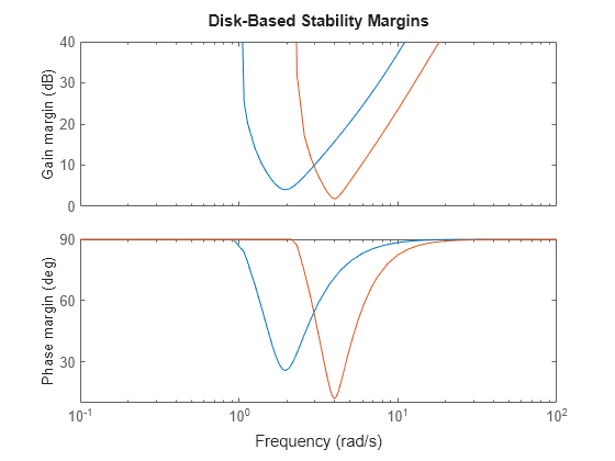
Compare the disk-based gain and phase margins of two open-loop responses on the same plot.

L1 = tf(25,[1 10 10 10]);
L2 = tf([1 100],[1 10 20 50]);
diskmarginplot(L1,L2)

MATLAB figure

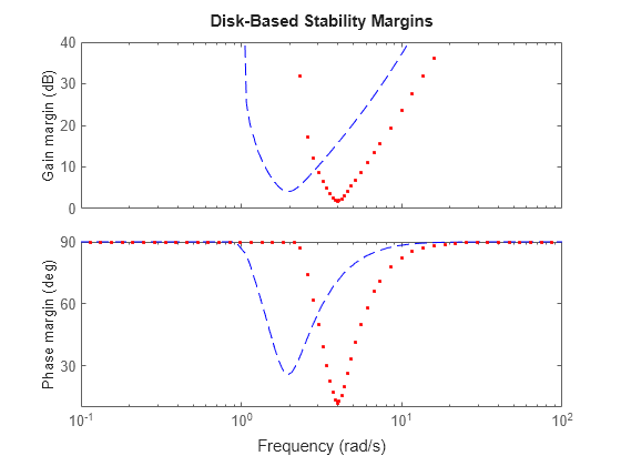
You can customize the appearance of the plots using the LineSpec argument. Plot the margins again, using a blue dashed line for L1 and red dots for L2.

diskmarginplot(L1,'b--',L2,'r.')

MATLAB figure

Combined Gain and Phase Variation

Open Live Script

The disk-based gain margins returned by diskmargin assume no phase variation, and the phase margins assume no gain variation. In practice, systems experience both gain and phase variation at the same time. Disk-margin analysis accounts for such simultaneous gain and phase variation.

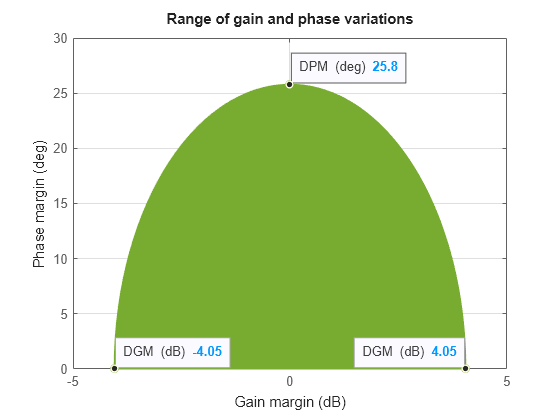
Compute the disk-based gain and phase margins of a system. Then, use diskmarginplot to visualize the corresponding allowed ranges of simultaneous gain and phase variation.

L = tf(25,[1 10 10 10]);
DM = diskmargin(L);
DGM = DM.GainMargin

DGM = 1×2

    0.6273    1.5942

DPM = DM.PhaseMargin

DPM = 1×2

  -25.8017   25.8017

diskmarginplot(DGM)

MATLAB figure

The shaded region in the plot shows the range of simultaneous gain and phase variations that preserve the stability of the closed-loop system feedback(L,1). When there is no phase variation, the system can tolerate the full gain-variation range DGM, from –4 dB to 4 dB. If the phase is allowed to vary by about ±20 degrees, the allowable gain-variation range drops to about –2.5 dB to 2 dB. At the full phase-variation range of ±26 degrees, the system can tolerate no gain variation.

To visualize multiple ranges on the same plot, combine them into a two-column vector. For instance, compute the disk margins of L with positive and negative skew and plot all three ranges of variation together.

DMn = diskmargin(L,-2);
DGMn = DMn.GainMargin;
DMp = diskmargin(L,2);
DGMp = DMp.GainMargin;
DGMall = [DGMn;DGM;DGMp];
diskmarginplot(DGMall)

MATLAB figure

This plot shows that the feedback loop can tolerate larger gain and phase variations when the gain decreases. In other words, the loop stability is more sensitive to gain increase. For more information about how varying skew affects disk-based gain and phase margin estimates, see Stability Analysis Using Disk Margins.

Disk of Uncertainty Corresponding to Disk-Based Gain Margin

Open Live Script

Disk-based gain-margin analysis models gain and phase variation as an uncertain factor F, multiplying an open-loop gain L. (For details of this model, see Stability Analysis Using Disk Margins.) The stable range of gain and phase variations returned by the diskmargin command is equivalent to a disk of F values for which the closed loop is stable. When you obtain the disk-based gain and phase margins of a system, you can use diskmarginplot to visualize the corresponding disk of F values.

L = tf(25,[1 10 10 10]);
DM = diskmargin(L);
DGM = DM.GainMargin

DGM = 1×2

    0.6273    1.5942

diskmarginplot(DGM,'disk')

MATLAB figure

The plot shows the values of F in the complex plane, where the x-axis is the real part and the y-axis is the imaginary part. The disk-based gain margin DGM uniquely determines this disk and the corresponding disk-based phase margin, DPM.

Disk Model of Gain and Phase Variation

Open Live Script

The uncertainty disk F is parameterized by two values: α, which sets the size of the disk, and σ, which biases the gain variation toward gain increase or decrease. This parameterization is given by:

$F = \frac{1 + α [(1 - σ) / 2] δ}{1 - α [(1 + σ) / 2] δ}$ ,

where δ is a normalized uncertainty. (For details, see Stability Analysis Using Disk Margins.) For a given range of gain variation, you can use gm2dm to convert the disk-based gain margin DGM to the α and σ values that describe the corresponding disk. diskmarginplot can plot the F disk for a given α,σ pair.

DGM = [0.8,2]

DGM = 1×2

    0.8000    2.0000

[alpha,sigma] = gm2dm(DGM);
diskmarginplot(alpha,sigma,'disk')

MATLAB figure

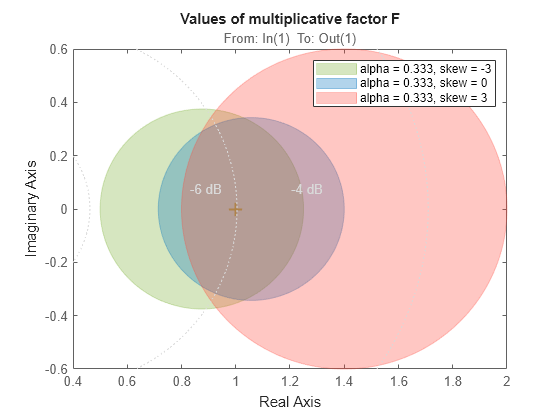
In this case, σ is greater than zero because the disk-based gain range DGM = [0.8,2] includes more gain increase than decrease. σ = 0 represents a gain that can increase as much as it can decrease. σ < 0 represents a range with more decrease than increase. Plot the F disk for different values of σ to see how the gain range (the diameter of the disk) varies with σ.

sigma = [-3,0,3];
diskmarginplot(alpha,sigma,'disk')

MATLAB figure

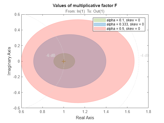
For a fixed σ, α controls the size of the disk, and hence the amount of modeled uncertainty. Plot the disk for several values of α at σ = 0.

sigma = 0;
alpha = [0.1,0.333,0.5];
diskmarginplot(alpha,sigma,'disk')

MATLAB figure

Nyquist Plot of Exclusion Disk

Open Live Script

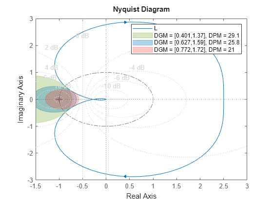
As described in Stability Analysis Using Disk Margins, for a given σ, the largest uncertainty disk F for which the closed-loop system feedback(L*F,1) remains stable can be interpreted as an exclusion region that the Nyquist curve of L cannot enter. For any value of σ, the exclusion disk contains the critical point (–1,0) and is tangent to the Nyquist curve. The skew adjusts the size and position of the tangent disks. You can use diskmarginplot to visualize these exclusion disks and superimpose them on the Nyquist curve of L.

Compute disk-based gain margins for a system using three different skew values, one corresponding to more gain increase than decrease (σ > 0), one corresponding to more gain decrease than increase (σ < 0), and one balanced (σ = 0).

L = tf(25,[1 10 10 10]);
DMdec = diskmargin(L,-2);
DGMdec = DMdec.GainMargin;
DM = diskmargin(L,0);
DGM = DM.GainMargin;
DMinc = diskmargin(L,2);
DGMinc= DMinc.GainMargin;

To view the corresponding exclusion regions, plot the Nyquist plots of L and hold the figure. Then use diskmarginplot with the 'nyquist' flag to add the exclusion regions to the plot.

nyquist(L)
hold on
diskmarginplot([DGMdec;DGM;DGMinc],'nyquist')
hold off

MATLAB figure

As σ increases from –2 to 2, the disks move to the right, and each disk provides lower estimates of the classical gain and phase margins.

Disk Margin Plot with Customized Appearance

Open Live Script

Plot the disk margins as a function of frequency of a system with the following open-loop response.

L = tf(25,[1 10 10 10]);

For the plot, specify the following attributes:

Frequency units: Hz
Gain margins on a log scale, in absolute units
Grid on

opts = diskmarginoptions;
opts.FreqUnits = 'Hz';
opts.MagScale = 'log';
opts.MagUnits = 'abs';
opts.grid = 'on';

diskmarginplot(L,opts)

MATLAB figure

Input Arguments

collapse all

`L` — Open-loop response
dynamic system model | model array

Open-loop response, specified as a dynamic system model. L can be SISO or MIMO, as long as it has the same number of inputs and outputs. diskmarginplot plots the disk-based gain and phase margins for the negative-feedback closed-loop system feedback(L,eye(N)).

To plot the margins of the positive feedback system feedback(L,eye(N),+1), use diskmargin(-L).

If L is an uncertain state-space model (uss or genss with uncertain blocks), then diskmarginplot plots the margins of random samples of L. To visualize the worst-case stability margins of an uncertain system, use wcdiskmarginplot.

If L is a frequency-response data model (such as frd), then diskmarginplot plots the margins at each frequency represented in the model.

If L is a model array, then diskmarginplot plots the margins for all models in the array on the same axis and in the same line style.

`LineSpec` — Line style, marker, and color
character vector | string

Line style, marker, and color, specified as a string or vector of one, two, or three characters. The characters can appear in any order. You do not need to specify all three characteristics (line style, marker, and color). For example, if you omit the line style and specify the marker, then the plot shows only the marker and no line. For more information about configuring this argument, see the LineSpec input argument of the plot function.

Example: 'r--' specifies a red dashed line

Example: '*b' specifies blue asterisk markers

Example: 'y' specifies a yellow line

`sigma` — Skew
0 (default) | real scalar | vector

Skew of uncertainty region used to compute the stability margins, specified as a real scalar or vector (for diskmarginplot(alpha,sigma) plots only).

This parameter biases the uncertainty used to model gain and phase variations toward gain increase or gain decrease.

The default sigma = 0 uses a balanced model of gain variation in a range [gmin,gmax], with gmin = 1/gmax.
Positive sigma uses a model with more gain increase than decrease (gmin > 1/gmax).
Negative sigma uses a model with more gain decrease than increase (gmin < 1/gmax).

For more detailed information about how the choice of sigma affects the margin computation, see Stability Analysis Using Disk Margins.

Skew in `diskmargin(L,sigma)` Syntax

When plotting the gain margins of a dynamic system versus frequency, use the default sigma = 0 to get unbiased estimates of gain and phase margins. For sigma = 0, the disk-based gain margin at each frequency is ±GM, where GM is the value shown in the plot in dB.

If you have used diskmargin to obtain disk-based margins with some particular sigma, you can use this syntax to see the frequency dependence of the margins at that sigma value. For sigma ≠ 0, the plotted value is GM = min(gmax,1/max(0,gmin)). In other words, the plot shows the largest amount of gain change [1/GM,GM] that fits within the disk-based gain margin [gmin,gmax] of the system at the specified sigma.

For the syntax diskmarginplot(L,sigma), the skew sigma must be a scalar.

Skew in `diskmargin(alpha,sigma)` Syntax

In the syntax diskmargin(alpha,sigma), the function plots the uncertainty disk parameterized by the values alpha and sigma (see Stability Analysis Using Disk Margins). To convert between disk-based gain margins and alpha, sigma parameterization, use dm2gm and gm2dm. For this syntax, diskmarginplot enforces the relation alpha*abs(1+sigma) < 2.

For this syntax, the skew sigma can be a vector, allowing you to compare multiple disks on the same plot. If alpha is a scalar and sigma is a vector, then the plot shows the disks corresponding to the pairs alpha,sigma_k for each entry in sigma. If both alpha and sigma are vectors, then the plot shows the disks for the pairs alpha1,sigma1;...;alphaN,sigmaN.

`w` — Frequencies
`{wmin,wmax}` | vector

Frequencies at which to plot stability margins, specified as the cell array {wmin,wmax} or as a vector of frequency values.

If w is a cell array of the form {wmin,wmax}, then the plot shows the margins at frequencies between wmin and wmax.
If w is a vector of frequencies, then the plot shows the margins at each specified frequency. For example, use logspace to generate a row vector with logarithmically spaced frequency values.

Specify frequencies in units of rad/TimeUnit, where TimeUnit is the TimeUnit property of L.

`opts` — Plot options
`diskmarginplot` options set

Plot options, specified as a diskmarginplot options set that you create with diskmarginoptions. Elements that you can customize include plot title, axes labels, and grids.

`DGM` — Disk-based gain margin
two-element vector | two-column matrix | scalar | column vector

Disk-based gain margin, specified as a scalar, a two-element vector of the form [gmin,gmax], or a two-column matrix of the form [gmin1,gmax1; ...; gminN,gmaxN].

Use a two-element vector, DGM = [gmin,gmax] to plot the allowable range of simultaneous gain and phase variations corresponding to the disk-based gain margin [gmin,gmax]. You can obtain [gmin,gmax] in the GainMargin field of the output structures of the diskmargin command. You can also obtain [gmin,gmax] from classical gain and phase margins using getDGM.

Using a scalar DGM is equivalent to specifying the symmetric gain margin [1/DGM,DGM].

To show the ranges of several disk-based gain margins on the same plot, use DGM = [gmin1,gmax1;...;gminN,gmaxN]. For symmetric gain margins of the form [1/gmax,gmax], you can use a column vector of the form [gmax1;gmax2;...;gmaxN].

`alpha` — Size of gain and phase variation
scalar | vector

Size of modeled gain and phase variation, specified as a scalar or vector. Disk-based gain-margin analysis models gain and phase variation as a multiplicative uncertainty F, which is a disk of values containing F = 1, corresponding to the nominal value of the system. The disk is parameterized by alpha, which sets the size of the disk, and sigma, which biases the gain variation toward gain increase or decrease. (For details of this model, see Stability Analysis Using Disk Margins.)

diskmarginplot lets you plot the disk F or the region of gain and phase variations represented by particular alpha,sigma pairs. For the syntax diskmarginplot(alpha,sigma), the disk size alpha can be a vector. If alpha is a vector and sigma is a scalar, then the plot shows the regions corresponding to the pairs alpha_k,sigma for each entry in alpha. If both alpha and sigma are vectors, then the plot shows the regions for the pairs alpha1,sigma1;...;alphaN,sigmaN.

diskmarginplot enforces the relation alpha*abs(1+sigma) < 2. To convert between disk-based gain margins and alpha, sigma parameterization, use dm2gm and gm2dm.

`AX` — Axes handle
`axes` object | `UIAxes` object

Axes handle, specified as an axes object or a UIaxes object. Use this argument to specify axes when creating apps in Develop Apps Using App Designer.

References

[1] Seiler, Peter, Andrew Packard, and Pascal Gahinet. “An Introduction to Disk Margins [Lecture Notes].” IEEE Control Systems Magazine 40, no. 5 (October 2020): 78–95.

Version History

Introduced in R2020a

diskmarginplot

Syntax

Description

Margins as a Function of Frequency

Range of Gain and Phase Variations

Plot on Specified Axes

Examples

Plot Gain and Phase Margins Versus Frequency

Compare Disk Margins of Multiple Systems

Combined Gain and Phase Variation

Disk of Uncertainty Corresponding to Disk-Based Gain Margin

Disk Model of Gain and Phase Variation

Nyquist Plot of Exclusion Disk

Disk Margin Plot with Customized Appearance

Input Arguments

`L` — Open-loop response
dynamic system model | model array

`LineSpec` — Line style, marker, and color
character vector | string

`sigma` — Skew
0 (default) | real scalar | vector

Skew in `diskmargin(L,sigma)` Syntax

Skew in `diskmargin(alpha,sigma)` Syntax

`w` — Frequencies
`{wmin,wmax}` | vector

`opts` — Plot options
`diskmarginplot` options set

`DGM` — Disk-based gain margin
two-element vector | two-column matrix | scalar | column vector

`alpha` — Size of gain and phase variation
scalar | vector

`AX` — Axes handle
`axes` object | `UIAxes` object

References

Version History

See Also

Topics

diskmarginplot

Syntax

Description

Margins as a Function of Frequency

Range of Gain and Phase Variations

Plot on Specified Axes

Examples

Plot Gain and Phase Margins Versus Frequency

Compare Disk Margins of Multiple Systems

Combined Gain and Phase Variation

Disk of Uncertainty Corresponding to Disk-Based Gain Margin

Disk Model of Gain and Phase Variation

Nyquist Plot of Exclusion Disk

Disk Margin Plot with Customized Appearance

Input Arguments

L — Open-loop response dynamic system model | model array

LineSpec — Line style, marker, and color character vector | string

sigma — Skew 0 (default) | real scalar | vector

Skew in diskmargin(L,sigma) Syntax

Skew in diskmargin(alpha,sigma) Syntax

w — Frequencies {wmin,wmax} | vector

opts — Plot options diskmarginplot options set

DGM — Disk-based gain margin two-element vector | two-column matrix | scalar | column vector

alpha — Size of gain and phase variation scalar | vector

AX — Axes handle axes object | UIAxes object

References

Version History

See Also

Topics

`L` — Open-loop response
dynamic system model | model array

`LineSpec` — Line style, marker, and color
character vector | string

`sigma` — Skew
0 (default) | real scalar | vector

Skew in `diskmargin(L,sigma)` Syntax

Skew in `diskmargin(alpha,sigma)` Syntax

`w` — Frequencies
`{wmin,wmax}` | vector

`opts` — Plot options
`diskmarginplot` options set

`DGM` — Disk-based gain margin
two-element vector | two-column matrix | scalar | column vector

`alpha` — Size of gain and phase variation
scalar | vector

`AX` — Axes handle
`axes` object | `UIAxes` object